3.3 Recursive Data Structures
In Chapter 2, we introduced the notion of a pair as a primitive mechanism for glueing together two objects into one. We showed that a pair can be implemented using a built-in tuple. The closure property of pairs indicated that either element of a pair could itself be a pair.
This closure property allowed us to implement the recursive list data abstraction, which served as our first type of sequence. Recursive lists are most naturally manipulated using recursive functions, as their name and structure would suggest. In this section, we discuss functions for creating and manipulating recursive lists and other recursive data structures.
3.3.1 Processing Recursive Lists
Recall that the recursive list abstract data type represented a list as a first element and the rest of the list. We previously implemented recursive lists using functions, but at this point we can re-implement them using a class. Below, the length (__len__) and element selection (__getitem__) functions are written recursively to demonstrate typical patterns for processing recursive lists.
>>> class Rlist(object):
        """A recursive list consisting of a first element and the rest."""
        class EmptyList(object):
            def __len__(self):
                return 0
        empty = EmptyList()
        def __init__(self, first, rest=empty):
            self.first = first
            self.rest = rest
        def __repr__(self):
            args = repr(self.first)
            if self.rest is not Rlist.empty:
                args += ', {0}'.format(repr(self.rest))
            return 'Rlist({0})'.format(args)
        def __len__(self):
            return 1 + len(self.rest)
        def __getitem__(self, i):
            if i == 0:
                return self.first
            return self.rest[i-1]
The definitions of __len__ and __getitem__ are in fact recursive, although not explicitly so. The built-in Python function len looks for a method called __len__ when applied to a user-defined object argument. Likewise, the subscript operator looks for a method called __getitem__. Thus, these definitions will end up calling themselves. Recursive calls on the rest of the list are a ubiquitous pattern in recursive list processing. This class definition of a recursive list interacts properly with Python's built-in sequence and printing operations.
>>> s = Rlist(1, Rlist(2, Rlist(3)))
>>> s.rest
Rlist(2, Rlist(3))
>>> len(s)
3
>>> s[1]
2
Operations that create new lists are particularly straightforward to express using recursion. For example, we can define a function extend_rlist, which takes two recursive lists as arguments and combines the elements of both into a new list.
>>> def extend_rlist(s1, s2):
        if s1 is Rlist.empty:
            return s2
        return Rlist(s1.first, extend_rlist(s1.rest, s2))
>>> extend_rlist(s.rest, s)
Rlist(2, Rlist(3, Rlist(1, Rlist(2, Rlist(3)))))
Likewise, mapping a function over a recursive list exhibits a similar pattern.
>>> def map_rlist(s, fn):
        if s is Rlist.empty:
            return s
        return Rlist(fn(s.first), map_rlist(s.rest, fn))
>>> map_rlist(s, square)
Rlist(1, Rlist(4, Rlist(9)))
Filtering includes an additional conditional statement, but otherwise has a similar recursive structure.
>>> def filter_rlist(s, fn):
        if s is Rlist.empty:
            return s
        rest = filter_rlist(s.rest, fn)
        if fn(s.first):
            return Rlist(s.first, rest)
        return rest
>>> filter_rlist(s, lambda x: x % 2 == 1)
Rlist(1, Rlist(3))
Recursive implementations of list operations do not, in general, require local assignment or while statements. Instead, recursive lists are taken apart and constructed incrementally as a consequence of function application. As a result, they have linear orders of growth in both the number of steps and space required.
3.3.2 Hierarchical Structures
Hierarchical structures result from the closure property of data, which asserts for example that tuples can contain other tuples. For instance, consider this nested representation of the numbers 1 through 4.
>>> ((1, 2), 3, 4)
((1, 2), 3, 4)
This tuple is a length-three sequence, of which the first element is itself a tuple. A box-and-pointer diagram of this nested structure shows that it can also be thought of as a tree with four leaves, each of which is a number.
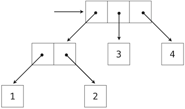
In a tree, each subtree is itself a tree. As a base condition, any bare element that is not a tuple is itself a simple tree, one with no branches. That is, the numbers are all trees, as is the pair (1, 2) and the structure as a whole.
Recursion is a natural tool for dealing with tree structures, since we can often reduce operations on trees to operations on their branches, which reduce in turn to operations on the branches of the branches, and so on, until we reach the leaves of the tree. As an example, we can implement a count_leaves function, which returns the total number of leaves of a tree.
>>> def count_leaves(tree):
        if type(tree) != tuple:
            return 1
        return sum(map(count_leaves, tree))
>>> t = ((1, 2), 3, 4)
>>> count_leaves(t)
4
>>> big_tree = ((t, t), 5)
>>> big_tree
((((1, 2), 3, 4), ((1, 2), 3, 4)), 5)
>>> count_leaves(big_tree)
9
Just as map is a powerful tool for dealing with sequences, mapping and recursion together provide a powerful general form of computation for manipulating trees. For instance, we can square all leaves of a tree using a higher-order recursive function map_tree that is structured quite similarly to count_leaves.
>>> def map_tree(tree, fn):
        if type(tree) != tuple:
            return fn(tree)
        return tuple(map_tree(branch, fn) for branch in tree)
>>> map_tree(big_tree, square)
((((1, 4), 9, 16), ((1, 4), 9, 16)), 25)
Internal values. The trees described above have values only at the leaves. Another common representation of tree-structured data has values for the internal nodes of the tree as well. We can represent such trees using a class.
>>> class Tree(object):
        def __init__(self, entry, left=None, right=None):
            self.entry = entry
            self.left = left
            self.right = right
        def __repr__(self):
            args = repr(self.entry)
            if self.left or self.right:
                args += ', {0}, {1}'.format(repr(self.left), repr(self.right))
            return 'Tree({0})'.format(args)
The Tree class can represent, for instance, the values computed in an expression tree for the recursive implementation of fib, the function for computing Fibonacci numbers. The function fib_tree(n) below returns a Tree that has the nth Fibonacci number as its entry and a trace of all previously computed Fibonacci numbers within its branches.
>>> def fib_tree(n):
        """Return a Tree that represents a recursive Fibonacci calculation."""
        if n == 1:
            return Tree(0)
        if n == 2:
            return Tree(1)
        left = fib_tree(n-2)
        right = fib_tree(n-1)
        return Tree(left.entry + right.entry, left, right)
>>> fib_tree(5)
Tree(3, Tree(1, Tree(0), Tree(1)), Tree(2, Tree(1), Tree(1, Tree(0), Tree(1))))
This example shows that expression trees can be represented programmatically using tree-structured data. This connection between nested expressions and tree-structured data type plays a central role in our discussion of designing interpreters later in this chapter.
3.3.3 Sets
In addition to the list, tuple, and dictionary, Python has a fourth built-in container type called a set. Set literals follow the mathematical notation of elements enclosed in braces. Duplicate elements are removed upon construction. Sets are unordered collections, and so the printed ordering may differ from the element ordering in the set literal.
>>> s = {3, 2, 1, 4, 4}
>>> s
{1, 2, 3, 4}
Python sets support a variety of operations, including membership tests, length computation, and the standard set operations of union and intersection
>>> 3 in s
True
>>> len(s)
4
>>> s.union({1, 5})
{1, 2, 3, 4, 5}
>>> s.intersection({6, 5, 4, 3})
{3, 4}
In addition to union and intersection, Python sets support several other methods. The predicates isdisjoint, issubset, and issuperset provide set comparison. Sets are mutable, and can be changed one element at a time using add, remove, discard, and pop. Additional methods provide multi-element mutations, such as clear and update. The Python documentation for sets should be sufficiently intelligible at this point of the course to fill in the details.
Implementing sets. Abstractly, a set is a collection of distinct objects that supports membership testing, union, intersection, and adjunction. Adjoining an element and a set returns a new set that contains all of the original set's elements along with the new element, if it is distinct. Union and intersection return the set of elements that appear in either or both sets, respectively. As with any data abstraction, we are free to implement any functions over any representation of sets that provides this collection of behaviors.
In the remainder of this section, we consider three different methods of implementing sets that vary in their representation. We will characterize the efficiency of these different representations by analyzing the order of growth of set operations. We will use our Rlist and Tree classes from earlier in this section, which allow for simple and elegant recursive solutions for elementary set operations.
Sets as unordered sequences. One way to represent a set is as a sequence in which no element appears more than once. The empty set is represented by the empty sequence. Membership testing walks recursively through the list.
>>> def empty(s):
        return s is Rlist.empty
>>> def set_contains(s, v):
        """Return True if and only if set s contains v."""
        if empty(s):
            return False
        elif s.first == v:
            return True
        return set_contains(s.rest, v)
>>> s = Rlist(1, Rlist(2, Rlist(3)))
>>> set_contains(s, 2)
True
>>> set_contains(s, 5)
False
This implementation of set_contains requires (\Theta(n)) time to test membership of an element, where (n) is the size of the set s. Using this linear-time function for membership, we can adjoin an element to a set, also in linear time.
>>> def adjoin_set(s, v):
        """Return a set containing all elements of s and element v."""
        if set_contains(s, v):
            return s
        return Rlist(v, s)
>>> t = adjoin_set(s, 4)
>>> t
Rlist(4, Rlist(1, Rlist(2, Rlist(3))))
In designing a representation, one of the issues with which we should be concerned is efficiency. Intersecting two sets set1 and set2 also requires membership testing, but this time each element of set1 must be tested for membership in set2, leading to a quadratic order of growth in the number of steps, (\Theta(n^2)), for two sets of size (n).
>>> def intersect_set(set1, set2):
        """Return a set containing all elements common to set1 and set2."""
        return filter_rlist(set1, lambda v: set_contains(set2, v))
>>> intersect_set(t, map_rlist(s, square))
Rlist(4, Rlist(1))
When computing the union of two sets, we must be careful not to include any element twice. The union_set function also requires a linear number of membership tests, creating a process that also includes (\Theta(n^2)) steps.
>>> def union_set(set1, set2):
        """Return a set containing all elements either in set1 or set2."""
        set1_not_set2 = filter_rlist(set1, lambda v: not set_contains(set2, v))
        return extend_rlist(set1_not_set2, set2)
>>> union_set(t, s)
Rlist(4, Rlist(1, Rlist(2, Rlist(3))))
Sets as ordered tuples. One way to speed up our set operations is to change the representation so that the set elements are listed in increasing order. To do this, we need some way to compare two objects so that we can say which is bigger. In Python, many different types of objects can be compared using < and > operators, but we will concentrate on numbers in this example. We will represent a set of numbers by listing its elements in increasing order.
One advantage of ordering shows up in set_contains: In checking for the presence of an object, we no longer have to scan the entire set. If we reach a set element that is larger than the item we are looking for, then we know that the item is not in the set:
>>> def set_contains(s, v):
        if empty(s) or s.first > v:
            return False
        elif s.first == v:
            return True
        return set_contains(s.rest, v)
>>> set_contains(s, 0)
False
How many steps does this save? In the worst case, the item we are looking for may be the largest one in the set, so the number of steps is the same as for the unordered representation. On the other hand, if we search for items of many different sizes we can expect that sometimes we will be able to stop searching at a point near the beginning of the list and that other times we will still need to examine most of the list. On average we should expect to have to examine about half of the items in the set. Thus, the average number of steps required will be about (\frac{n}{2}). This is still (\Theta(n)) growth, but it does save us, on average, a factor of 2 in the number of steps over the previous implementation.
We can obtain a more impressive speedup by re-implementing intersect_set. In the unordered representation, this operation required (\Theta(n^2)) steps because we performed a complete scan of set2 for each element of set1. But with the ordered representation, we can use a more clever method. We iterate through both sets simultaneously, tracking an element e1 in set1 and e2 in set2. When e1 and e2 are equal, we include that element in the intersection.
Suppose, however, that e1 is less than e2. Since e2 is smaller than the remaining elements of set2, we can immediately conclude that e1 cannot appear anywhere in the remainder of set2 and hence is not in the intersection. Thus, we no longer need to consider e1; we discard it and proceed to the next element of set1. Similar logic advances through the elements of set2 when e2 < e1. Here is the function:
>>> def intersect_set(set1, set2):
        if empty(set1) or empty(set2):
            return Rlist.empty
        e1, e2 = set1.first, set2.first
        if e1 == e2:
            return Rlist(e1, intersect_set(set1.rest, set2.rest))
        elif e1 < e2:
            return intersect_set(set1.rest, set2)
        elif e2 < e1:
            return intersect_set(set1, set2.rest)
>>> intersect_set(s, s.rest)
Rlist(2, Rlist(3))
To estimate the number of steps required by this process, observe that in each step we shrink the size of at least one of the sets. Thus, the number of steps required is at most the sum of the sizes of set1 and set2, rather than the product of the sizes, as with the unordered representation. This is (\Theta(n)) growth rather than (\Theta(n^2)) -- a considerable speedup, even for sets of moderate size. For example, the intersection of two sets of size 100 will take around 200 steps, rather than 10,000 for the unordered representation.
Adjunction and union for sets represented as ordered sequences can also be computed in linear time. These implementations are left as an exercise.
Sets as binary trees. We can do better than the ordered-list representation by arranging the set elements in the form of a tree. We use the Tree class introduced previously. The entry of the root of the tree holds one element of the set. The entries within the left branch include all elements smaller than the one at the root. Entries in the right branch include all elements greater than the one at the root. The figure below shows some trees that represent the set {1, 3, 5, 7, 9, 11}. The same set may be represented by a tree in a number of different ways. The only thing we require for a valid representation is that all elements in the left subtree be smaller than the tree entry and that all elements in the right subtree be larger.

The advantage of the tree representation is this: Suppose we want to check whether a value v is contained in a set. We begin by comparing v with entry. If v is less than this, we know that we need only search the left subtree; if v is greater, we need only search the right subtree. Now, if the tree is "balanced," each of these subtrees will be about half the size of the original. Thus, in one step we have reduced the problem of searching a tree of size (n) to searching a tree of size (\frac{n}{2}). Since the size of the tree is halved at each step, we should expect that the number of steps needed to search a tree grows as (\Theta(\log n)). For large sets, this will be a significant speedup over the previous representations. This set_contains function exploits the ordering structure of the tree-structured set.
>>> def set_contains(s, v):
        if s is None:
            return False
        elif s.entry == v:
            return True
        elif s.entry < v:
            return set_contains(s.right, v)
        elif s.entry > v:
            return set_contains(s.left, v)
Adjoining an item to a set is implemented similarly and also requires (\Theta(\log n)) steps. To adjoin a value v, we compare v with entry to determine whether v should be added to the right or to the left branch, and having adjoined v to the appropriate branch we piece this newly constructed branch together with the original entry and the other branch. If v is equal to the entry, we just return the node. If we are asked to adjoin v to an empty tree, we generate a Tree that has v as the entry and empty right and left branches. Here is the function:
>>> def adjoin_set(s, v):
        if s is None:
            return Tree(v)
        if s.entry == v:
            return s
        if s.entry < v:
            return Tree(s.entry, s.left, adjoin_set(s.right, v))
        if s.entry > v:
            return Tree(s.entry, adjoin_set(s.left, v), s.right)
>>> adjoin_set(adjoin_set(adjoin_set(None, 2), 3), 1)
Tree(2, Tree(1), Tree(3))
Our claim that searching the tree can be performed in a logarithmic number of steps rests on the assumption that the tree is "balanced," i.e., that the left and the right subtree of every tree have approximately the same number of elements, so that each subtree contains about half the elements of its parent. But how can we be certain that the trees we construct will be balanced? Even if we start with a balanced tree, adding elements with adjoin_set may produce an unbalanced result. Since the position of a newly adjoined element depends on how the element compares with the items already in the set, we can expect that if we add elements "randomly" the tree will tend to be balanced on the average.
But this is not a guarantee. For example, if we start with an empty set and adjoin the numbers 1 through 7 in sequence we end up with a highly unbalanced tree in which all the left subtrees are empty, so it has no advantage over a simple ordered list. One way to solve this problem is to define an operation that transforms an arbitrary tree into a balanced tree with the same elements. We can perform this transformation after every few adjoin_set operations to keep our set in balance.
Intersection and union operations can be performed on tree-structured sets in linear time by converting them to ordered lists and back. The details are left as an exercise.
Python set implementation. The set type that is built into Python does not use any of these representations internally. Instead, Python uses a representation that gives constant-time membership tests and adjoin operations based on a technique called hashing, which is a topic for another course. Built-in Python sets cannot contain mutable data types, such as lists, dictionaries, or other sets. To allow for nested sets, Python also includes a built-in immutable frozenset class that shares methods with the set class but excludes mutation methods and operators.