八、如何实现线性回归

在上一课中，我们使用 scikit learn 的实现计算了糖尿病数据集的最小二乘线性回归。今天，我们将看看如何编写自己的实现。

起步

from sklearn import datasets, linear_model, metrics
from sklearn.model_selection import train_test_split
from sklearn.preprocessing import PolynomialFeatures
import math, scipy, numpy as np
from scipy import linalg

np.set_printoptions(precision=6)

data = datasets.load_diabetes()

feature_names=['age', 'sex', 'bmi', 'bp', 's1', 's2', 's3', 's4', 's5', 's6']

trn,test,y_trn,y_test = train_test_split(data.data, data.target, test_size=0.2)

trn.shape, test.shape

# ((353, 10), (89, 10))

def regr_metrics(act, pred):
    return (math.sqrt(metrics.mean_squared_error(act, pred)), 
    metrics.mean_absolute_error(act, pred))

sklearn 如何实现它

sklearn 是如何做到这一点的？通过检查源代码，你可以看到在密集的情况下，它调用scipy.linalg.lstqr，它调用 LAPACK 方法：

选项是'gelsd'，'gelsy'，'gelss'。默认值'gelsd'是个好的选择，但是，'gelsy'在许多问题上更快一些。'gelss'由于历史原因而使用。它通常更慢但是使用更少内存。

gelsd：使用 SVD 和分治方法
gelsy：使用 QR 分解
gelss：使用 SVD

Scipy 稀疏最小二乘

我们不会详细介绍稀疏版本的最小二乘法。如果你有兴趣，请参考以下信息：

Scipy 稀疏最小二乘使用称为 Golub 和 Kahan 双对角化的迭代方法。

Scipy 稀疏最小二乘源代码：预处理是减少迭代次数的另一种方法。如果有可能有效地求解相关系统M*x = b，其中M以某种有用的方式近似A（例如，M-A具有低秩或其元素相对于A的元素较小），则 LSQR 可以在系统A*M(inverse)*z = b更快地收敛。之后可以通过求解M * x = z来恢复x。

如果A是对称的，则不应使用 LSQR！替代方案是对称共轭梯度法（cg）和/或 SYMMLQ。 SYMMLQ 是对称 cg 的一种实现，适用于任何对称的A，并且比 LSQR 更快收敛。如果A是正定的，则存在对称 cg 的其他实现，每次迭代需要的工作量比 SYMMLQ 少一些（但需要相同的迭代次数）。

`linalg.lstqr`

sklearn 实现为我们添加一个常数项（因为对于我们正在学习的直线，y截距可能不是 0）。我们现在需要手工完成：

trn_int = np.c_[trn, np.ones(trn.shape[0])]
test_int = np.c_[test, np.ones(test.shape[0])]

由于linalg.lstsq允许我们指定，我们想要使用哪个 LAPACK 例程，让我们尝试它们并进行一些时间比较：

%timeit coef, _,_,_ = linalg.lstsq(trn_int, y_trn, lapack_driver="gelsd")

# 290 µs ± 9.24 µs per loop (mean ± std. dev. of 7 runs, 1000 loops each)

%timeit coef, _,_,_ = linalg.lstsq(trn_int, y_trn, lapack_driver="gelsy")

# 140 µs ± 91.7 ns per loop (mean ± std. dev. of 7 runs, 10000 loops each)

%timeit coef, _,_,_ = linalg.lstsq(trn_int, y_trn, lapack_driver="gelss")

# 199 µs ± 228 ns per loop (mean ± std. dev. of 7 runs, 1000 loops each)

朴素解法

回想一下，我们想找到 $\hat x$ ，来最小化：

$\big\vert\big\vert Ax - b \big\vert\big\vert_2$

另一种思考方式是，我们对向量b最接近A的子空间（称为A的范围）的地方感兴趣。这是b在A上的投影。由于 $b - A \hat x$ 必须垂直于A的子空间，我们可以看到：

$A^T (b - A\hat{x}) = 0$

使用了 $A^T$ 因为要相乘A和 $b - A\hat{x}$ 的每列。

这让我们得到正规方程：

$x = (A^TA)^{-1}A^T b$

def ls_naive(A, b):
     return np.linalg.inv(A.T @ A) @ A.T @ b

%timeit coeffs_naive = ls_naive(trn_int, y_trn)

# 45.8 µs ± 4.65 µs per loop (mean ± std. dev. of 7 runs, 10000 loops each)

coeffs_naive = ls_naive(trn_int, y_trn)
regr_metrics(y_test, test_int @ coeffs_naive)

# (57.94102134545707, 48.053565198516438)

正规方程（Cholesky）

正规方程：

$A^TA x = A^T b$

如果A具有满秩，则伪逆 $(A^TA)^{-1}A^T$ 是正方形，埃尔米特正定矩阵。解决这种系统的标准方法是 Cholesky 分解，它找到上三角形R，满足 $A^TA = R^TR$ 。

以下步骤基于 Trefethen 的算法 11.1：

A = trn_int

b = y_trn

AtA = A.T @ A
Atb = A.T @ b

警告：对于Cholesky，Numpy 和 Scipy 默认为不同的上/下三角。

R = scipy.linalg.cholesky(AtA)

np.set_printoptions(suppress=True, precision=4)
R

'''
array([[  0.9124,   0.1438,   0.1511,   0.3002,   0.2228,   0.188 ,
         -0.051 ,   0.1746,   0.22  ,   0.2768,  -0.2583],
       [  0.    ,   0.8832,   0.0507,   0.1826,  -0.0251,   0.0928,
         -0.3842,   0.2999,   0.0911,   0.15  ,   0.4393],
       [  0.    ,   0.    ,   0.8672,   0.2845,   0.2096,   0.2153,
         -0.2695,   0.3181,   0.3387,   0.2894,  -0.005 ],
       [  0.    ,   0.    ,   0.    ,   0.7678,   0.0762,  -0.0077,
          0.0383,   0.0014,   0.165 ,   0.166 ,   0.0234],
       [  0.    ,   0.    ,   0.    ,   0.    ,   0.8288,   0.7381,
          0.1145,   0.4067,   0.3494,   0.158 ,  -0.2826],
       [  0.    ,   0.    ,   0.    ,   0.    ,   0.    ,   0.3735,
         -0.3891,   0.2492,  -0.3245,  -0.0323,  -0.1137],
       [  0.    ,   0.    ,   0.    ,   0.    ,   0.    ,   0.    ,
          0.6406,  -0.511 ,  -0.5234,  -0.172 ,  -0.9392],
       [  0.    ,   0.    ,   0.    ,   0.    ,   0.    ,   0.    ,
          0.    ,   0.2887,  -0.0267,  -0.0062,   0.0643],
       [  0.    ,   0.    ,   0.    ,   0.    ,   0.    ,   0.    ,
          0.    ,   0.    ,   0.2823,   0.0636,   0.9355],
       [  0.    ,   0.    ,   0.    ,   0.    ,   0.    ,   0.    ,
          0.    ,   0.    ,   0.    ,   0.7238,   0.0202],
       [  0.    ,   0.    ,   0.    ,   0.    ,   0.    ,   0.    ,
          0.    ,   0.    ,   0.    ,   0.    ,  18.7319]])
'''

检查我们的分解：

np.linalg.norm(AtA - R.T @ R)

# 4.5140158187158533e-16

$A^T A x = A^T b \\ R^T R x = A^T b \\R^T w = A^T b \\R x = w$

w = scipy.linalg.solve_triangular(R, Atb, lower=False, trans='T')

检查我们的结果是否符合预期总是好的：（以防我们输入错误的参数，函数没有返回我们想要的东西，或者有时文档甚至过时）。

np.linalg.norm(R.T @ w - Atb)

# 1.1368683772161603e-13

coeffs_chol = scipy.linalg.solve_triangular(R, w, lower=False)

np.linalg.norm(R @ coeffs_chol - w)

# 6.861429794408013e-14

def ls_chol(A, b):
    R = scipy.linalg.cholesky(A.T @ A)
    w = scipy.linalg.solve_triangular(R, A.T @ b, trans='T')
    return scipy.linalg.solve_triangular(R, w)

%timeit coeffs_chol = ls_chol(trn_int, y_trn)

# 111 µs ± 272 ns per loop (mean ± std. dev. of 7 runs, 10000 loops each)

coeffs_chol = ls_chol(trn_int, y_trn)
regr_metrics(y_test, test_int @ coeffs_chol)

# (57.9410213454571, 48.053565198516438)

QR 分解

$A x = b \\ A = Q R \\ Q R x = b \\ R x = Q^T b$

def ls_qr(A,b):
    Q, R = scipy.linalg.qr(A, mode='economic')
    return scipy.linalg.solve_triangular(R, Q.T @ b)

%timeit coeffs_qr = ls_qr(trn_int, y_trn)

# 205 µs ± 264 ns per loop (mean ± std. dev. of 7 runs, 1000 loops each)

coeffs_qr = ls_qr(trn_int, y_trn)
regr_metrics(y_test, test_int @ coeffs_qr)

# (57.94102134545711, 48.053565198516452)

SVD

$A x = b \\ A = U \Sigma V \\ \Sigma V x = U^T b \\ \Sigma w = U^T b \\ x = V^T w$

SVD 给出伪逆。

def ls_svd(A,b):
    m, n = A.shape
    U, sigma, Vh = scipy.linalg.svd(A, full_matrices=False)
    w = (U.T @ b)/ sigma
    return Vh.T @ w

%timeit coeffs_svd = ls_svd(trn_int, y_trn)

# 1.11 ms ± 320 ns per loop (mean ± std. dev. of 7 runs, 1000 loops each)

%timeit coeffs_svd = ls_svd(trn_int, y_trn)

# 266 µs ± 8.49 µs per loop (mean ± std. dev. of 7 runs, 1000 loops each)

coeffs_svd = ls_svd(trn_int, y_trn)
regr_metrics(y_test, test_int @ coeffs_svd)

# (57.941021345457244, 48.053565198516687)

最小二乘回归的随机 Sketching 技巧

线性 Sketching（Woodruff）

抽取r×n随机矩阵S，r << n
计算S A和S b
找到回归SA x = Sb的精确解x

时间比较

import timeit
import pandas as pd

def scipylstq(A, b):
    return scipy.linalg.lstsq(A,b)[0]

row_names = ['Normal Eqns- Naive',
             'Normal Eqns- Cholesky', 
             'QR Factorization', 
             'SVD', 
             'Scipy lstsq']

name2func = {'Normal Eqns- Naive': 'ls_naive', 
             'Normal Eqns- Cholesky': 'ls_chol', 
             'QR Factorization': 'ls_qr',
             'SVD': 'ls_svd',
             'Scipy lstsq': 'scipylstq'}

m_array = np.array([100, 1000, 10000])
n_array = np.array([20, 100, 1000])

index = pd.MultiIndex.from_product([m_array, n_array], names=['# rows', '# cols'])

pd.options.display.float_format = '{:,.6f}'.format
df = pd.DataFrame(index=row_names, columns=index)
df_error = pd.DataFrame(index=row_names, columns=index)

# %%prun
for m in m_array:
    for n in n_array:
        if m >= n:        
            x = np.random.uniform(-10,10,n)
            A = np.random.uniform(-40,40,[m,n])   # removed np.asfortranarray
            b = np.matmul(A, x) + np.random.normal(0,2,m)
            for name in row_names:
                fcn = name2func[name]
                t = timeit.timeit(fcn + '(A,b)', number=5, globals=globals())
                df.set_value(name, (m,n), t)
                coeffs = locals()[fcn](A, b)
                reg_met = regr_metrics(b, A @ coeffs)
                df_error.set_value(name, (m,n), reg_met[0])

df

# rows	100			1000			10000
# cols	20	100	1000	20	100	1000	20	100	1000
Normal Eqns- Naive	0.001276	0.003634	NaN	0.000960	0.005172	0.293126	0.002226	0.021248	1.164655
Normal Eqns- Cholesky	0.001660	0.003958	NaN	0.001665	0.004007	0.093696	0.001928	0.010456	0.399464
QR Factorization	0.002174	0.006486	NaN	0.004235	0.017773	0.213232	0.019229	0.116122	2.208129
SVD	0.003880	0.021737	NaN	0.004672	0.026950	1.280490	0.018138	0.130652	3.433003
Scipy lstsq	0.004338	0.020198	NaN	0.004320	0.021199	1.083804	0.012200	0.088467	2.134780

df_error

# rows	100			1000			10000
# cols	20	100	1000	20	100	1000	20	100	1000
Normal Eqns- Naive	1.702742	0.000000	NaN	1.970767	1.904873	0.000000	1.978383	1.980449	1.884440
Normal Eqns- Cholesky	1.702742	0.000000	NaN	1.970767	1.904873	0.000000	1.978383	1.980449	1.884440
QR Factorization	1.702742	0.000000	NaN	1.970767	1.904873	0.000000	1.978383	1.980449	1.884440
SVD	1.702742	0.000000	NaN	1.970767	1.904873	0.000000	1.978383	1.980449	1.884440
Scipy lstsq	1.702742	0.000000	NaN	1.970767	1.904873	0.000000	1.978383	1.980449	1.884440

store = pd.HDFStore('least_squares_results.h5')
store['df'] = df

'''
C:\Users\rache\Anaconda3\lib\site-packages\IPython\core\interactiveshell.py:2881: PerformanceWarning: 
your performance may suffer as PyTables will pickle object types that it cannot
map directly to c-types [inferred_type->floating,key->block0_values] [items->[(100, 20), (100, 100), (100, 1000), (1000, 20), (1000, 100), (1000, 1000), (5000, 20), (5000, 100), (5000, 1000)]]

  exec(code_obj, self.user_global_ns, self.user_ns)
'''

注解

我用魔术指令%prun来测量我的代码。

替代方案：最小绝对偏差（L1 回归）

异常值的敏感度低于最小二乘法。
没有闭式解，但可以通过线性规划解决。

条件作用和稳定性

条件数

条件数是一个指标，衡量输入的小变化导致输出变化的程度。

问题：为什么我们在数值线性代数中，关心输入的小变化的相关行为？

相对条件数由下式定义：

$\kappa = \sup_{\delta x} \frac{\|\delta f\|}{\| f(x) \|}\bigg/ \frac{\| \delta x \|}{\| x \|}$

其中 $\delta x$ 是无穷小。

根据 Trefethen（第 91 页），如果κ很小（例如 1, 10, 10^2），问题是良态的，如果κ很大（例如10^6, 10^16），那么问题是病态的。

条件作用：数学问题的扰动行为（例如最小二乘）

稳定性：用于在计算机上解决该问题的算法的扰动行为（例如，最小二乘算法，householder，回代，高斯消除）

条件作用的例子

计算非对称矩阵的特征值的问题通常是病态的。

A = [[1, 1000], [0, 1]]
B = [[1, 1000], [0.001, 1]]

wA, vrA = scipy.linalg.eig(A)
wB, vrB = scipy.linalg.eig(B)

wA, wB

'''
(array([ 1.+0.j,  1.+0.j]),
 array([  2.00000000e+00+0.j,  -2.22044605e-16+0.j]))
'''

矩阵的条件数

乘积 $\| A\| \|A^{-1} \|$ 经常出现，它有自己的名字：A的条件数。注意，通常我们谈论问题的条件作用，而不是矩阵。

A的条件数涉及：

给定Ax = b中的A和x，计算b
给定Ax = b中的A和b，计算x

未交待清楚的事情

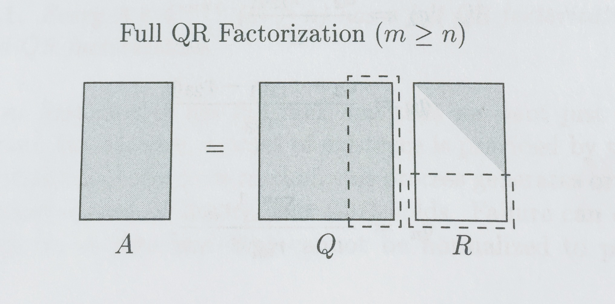
完整和简化分解

SVD

来自 Trefethen 的图：

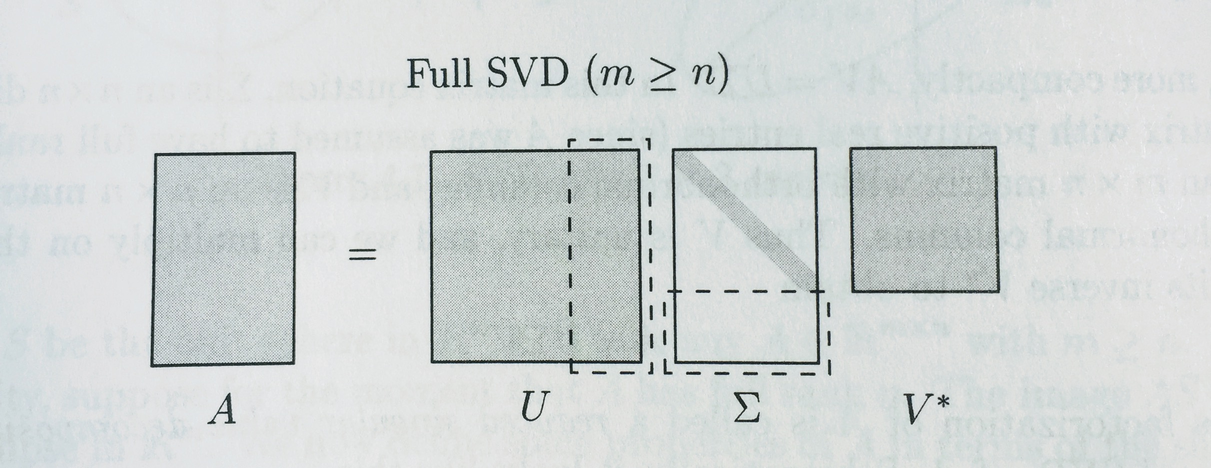
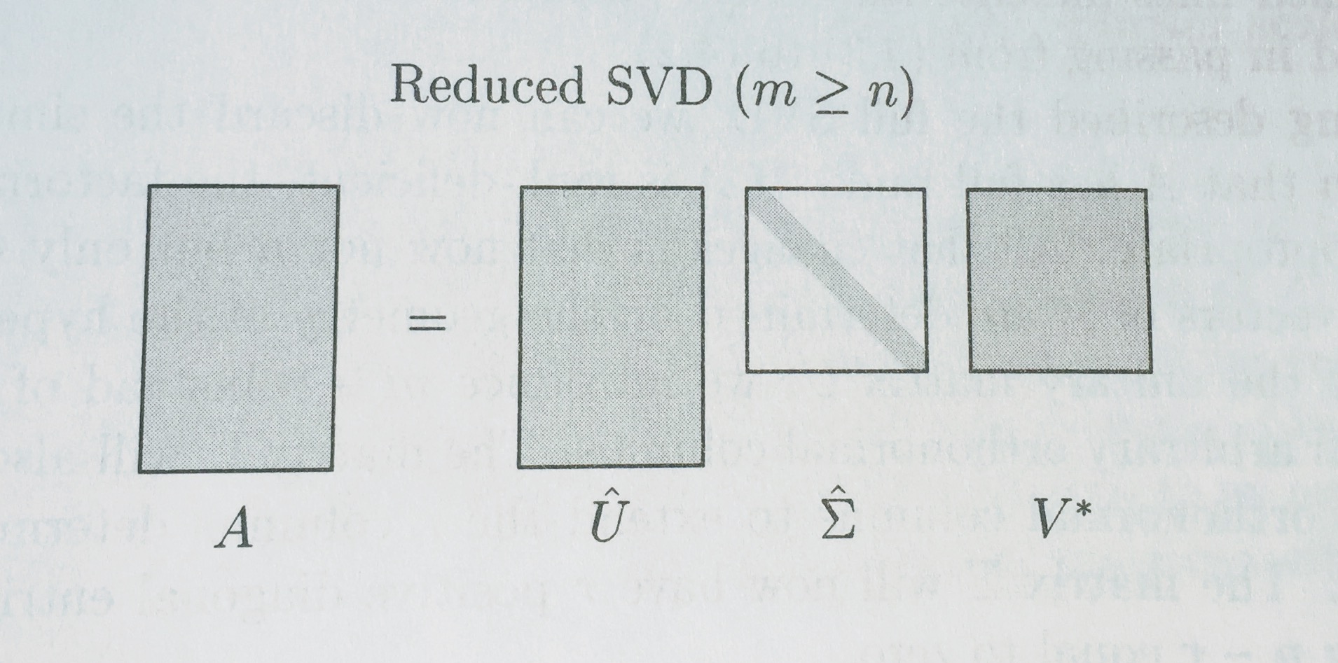
对于所有矩阵，QR 分解都存在

与 SVD 一样，有 QR 分解的完整版和简化版。

矩阵的逆是不稳定的

from scipy.linalg import hilbert

n = 5
hilbert(n)

'''
array([[ 1.    ,  0.5   ,  0.3333,  0.25  ,  0.2   ],
       [ 0.5   ,  0.3333,  0.25  ,  0.2   ,  0.1667],
       [ 0.3333,  0.25  ,  0.2   ,  0.1667,  0.1429],
       [ 0.25  ,  0.2   ,  0.1667,  0.1429,  0.125 ],
       [ 0.2   ,  0.1667,  0.1429,  0.125 ,  0.1111]])
'''

n = 14
A = hilbert(n)
x = np.random.uniform(-10,10,n)
b = A @ x

A_inv = np.linalg.inv(A)

np.linalg.norm(np.eye(n) - A @ A_inv)

# 5.0516495470543212

np.linalg.cond(A)

# 2.2271635826494112e+17

A @ A_inv

'''
array([[ 1.    ,  0.    , -0.0001,  0.0005, -0.0006,  0.0105, -0.0243,
         0.1862, -0.6351,  2.2005, -0.8729,  0.8925, -0.0032, -0.0106],
       [ 0.    ,  1.    , -0.    ,  0.    ,  0.0035,  0.0097, -0.0408,
         0.0773, -0.0524,  1.6926, -0.7776, -0.111 , -0.0403, -0.0184],
       [ 0.    ,  0.    ,  1.    ,  0.0002,  0.0017,  0.0127, -0.0273,
         0.    ,  0.    ,  1.4688, -0.5312,  0.2812,  0.0117,  0.0264],
       [ 0.    ,  0.    , -0.    ,  1.0005,  0.0013,  0.0098, -0.0225,
         0.1555, -0.0168,  1.1571, -0.9656, -0.0391,  0.018 , -0.0259],
       [-0.    ,  0.    , -0.    ,  0.0007,  1.0001,  0.0154,  0.011 ,
        -0.2319,  0.5651, -0.2017,  0.2933, -0.6565,  0.2835, -0.0482],
       [ 0.    , -0.    ,  0.    , -0.0004,  0.0059,  0.9945, -0.0078,
        -0.0018, -0.0066,  1.1839, -0.9919,  0.2144, -0.1866,  0.0187],
       [-0.    ,  0.    , -0.    ,  0.0009, -0.002 ,  0.0266,  0.974 ,
        -0.146 ,  0.1883, -0.2966,  0.4267, -0.8857,  0.2265, -0.0453],
       [ 0.    ,  0.    , -0.    ,  0.0002,  0.0009,  0.0197, -0.0435,
         1.1372, -0.0692,  0.7691, -1.233 ,  0.1159, -0.1766, -0.0033],
       [ 0.    ,  0.    , -0.    ,  0.0002,  0.    , -0.0018, -0.0136,
         0.1332,  0.945 ,  0.3652, -0.2478, -0.1682,  0.0756, -0.0212],
       [ 0.    , -0.    , -0.    ,  0.0003,  0.0038, -0.0007,  0.0318,
        -0.0738,  0.2245,  1.2023, -0.2623, -0.2783,  0.0486, -0.0093],
       [-0.    ,  0.    , -0.    ,  0.0004, -0.0006,  0.013 , -0.0415,
         0.0292, -0.0371,  0.169 ,  1.0715, -0.09  ,  0.1668, -0.0197],
       [ 0.    , -0.    ,  0.    ,  0.    ,  0.0016,  0.0062, -0.0504,
         0.1476, -0.2341,  0.8454, -0.7907,  1.4812, -0.15  ,  0.0186],
       [ 0.    , -0.    ,  0.    , -0.0001,  0.0022,  0.0034, -0.0296,
         0.0944, -0.1833,  0.6901, -0.6526,  0.2556,  0.8563,  0.0128],
       [ 0.    ,  0.    ,  0.    , -0.0001,  0.0018, -0.0041, -0.0057,
        -0.0374, -0.165 ,  0.3968, -0.2264, -0.1538, -0.0076,  1.005 ]])
'''

row_names = ['Normal Eqns- Naive',
             'QR Factorization', 
             'SVD', 
             'Scipy lstsq']

name2func = {'Normal Eqns- Naive': 'ls_naive', 
             'QR Factorization': 'ls_qr',
             'SVD': 'ls_svd',
             'Scipy lstsq': 'scipylstq'}

pd.options.display.float_format = '{:,.9f}'.format
df = pd.DataFrame(index=row_names, columns=['Time', 'Error'])

for name in row_names:
    fcn = name2func[name]
    t = timeit.timeit(fcn + '(A,b)', number=5, globals=globals())
    coeffs = locals()[fcn](A, b)
    df.set_value(name, 'Time', t)
    df.set_value(name, 'Error', regr_metrics(b, A @ coeffs)[0])

SVD 在这里最好

不要重新运行。

df

	Time	Error
Normal Eqns- Naive	0.001334339	3.598901966
QR Factorization	0.002166139	0.000000000
SVD	0.001556937	0.000000000
Scipy lstsq	0.001871590	0.000000000

即使A是稀疏的， $A^{-1}$ 通常是密集的。对于大型矩阵， $A^{-1}$ 放不进内存。

运行时间

矩阵求逆： $2n^3$
矩阵乘法： $n^3$
Cholesky： $1/3 n^3$
QR，Gram Schmidt： $2mn^2$ ， $m \ge n$ （Trefethen 第 8 章）
QR，Householder：2 $mn^2-2/3 n^3$ （Trefethen 第 10 章）
求解三角形系统： $n^2$

为什么 Cholesky 较快：

来源：斯坦福凸优化：数值线性代数背景幻灯片

QR 最优的一个案例

m=100
n=15
t=np.linspace(0, 1, m)

# 范德蒙矩阵
A=np.stack([t**i for i in range(n)], 1)
b=np.exp(np.sin(4*t))

# 这将使解决方案标准化为 1
b /= 2006.787453080206

from matplotlib import pyplot as plt
%matplotlib inline

plt.plot(t, b)

# [<matplotlib.lines.Line2D at 0x7fdfc1fa7eb8>]

检查我们得到了 1：

1 - ls_qr(A, b)[14]

# 1.4137685733217609e-07

不好的条件数：

kappa = np.linalg.cond(A); kappa

# 5.827807196683593e+17

row_names = ['Normal Eqns- Naive',
             'QR Factorization', 
             'SVD', 
             'Scipy lstsq']

name2func = {'Normal Eqns- Naive': 'ls_naive', 
             'QR Factorization': 'ls_qr',
             'SVD': 'ls_svd',
             'Scipy lstsq': 'scipylstq'}

pd.options.display.float_format = '{:,.9f}'.format
df = pd.DataFrame(index=row_names, columns=['Time', 'Error'])

for name in row_names:
    fcn = name2func[name]
    t = timeit.timeit(fcn + '(A,b)', number=5, globals=globals())
    coeffs = locals()[fcn](A, b)
    df.set_value(name, 'Time', t)
    df.set_value(name, 'Error', np.abs(1 - coeffs[-1]))

df

	Time	Error
Normal Eqns- Naive	0.001565099	1.357066025
QR Factorization	0.002632104	0.000000116
SVD	0.003503785	0.000000116
Scipy lstsq	0.002763502	0.000000116

通过正规方程求解最小二乘的解决方案通常是不稳定的，尽管对于小条件数的问题是稳定的。

低秩

m = 100
n = 10
x = np.random.uniform(-10,10,n)
A2 = np.random.uniform(-40,40, [m, int(n/2)])   # removed np.asfortranarray
A = np.hstack([A2, A2])

A.shape, A2.shape

# ((100, 10), (100, 5))

b = A @ x + np.random.normal(0,1,m)

row_names = ['Normal Eqns- Naive',
             'QR Factorization', 
             'SVD', 
             'Scipy lstsq']

name2func = {'Normal Eqns- Naive': 'ls_naive', 
             'QR Factorization': 'ls_qr',
             'SVD': 'ls_svd',
             'Scipy lstsq': 'scipylstq'}

pd.options.display.float_format = '{:,.9f}'.format
df = pd.DataFrame(index=row_names, columns=['Time', 'Error'])

for name in row_names:
    fcn = name2func[name]
    t = timeit.timeit(fcn + '(A,b)', number=5, globals=globals())
    coeffs = locals()[fcn](A, b)
    df.set_value(name, 'Time', t)
    df.set_value(name, 'Error', regr_metrics(b, A @ coeffs)[0])

df

	Time	Error
Normal Eqns- Naive	0.001227640	300.658979382
QR Factorization	0.002315920	0.876019803
SVD	0.001745647	1.584746056
Scipy lstsq	0.002067989	0.804750398

比较

比较我们的结果和上面：

df

# rows	100			1000			10000
# cols	20	100	1000	20	100	1000	20	100	1000
Normal Eqns- Naive	0.001276	0.003634	NaN	0.000960	0.005172	0.293126	0.002226	0.021248	1.164655
Normal Eqns- Cholesky	0.001660	0.003958	NaN	0.001665	0.004007	0.093696	0.001928	0.010456	0.399464
QR Factorization	0.002174	0.006486	NaN	0.004235	0.017773	0.213232	0.019229	0.116122	2.208129
SVD	0.003880	0.021737	NaN	0.004672	0.026950	1.280490	0.018138	0.130652	3.433003
Scipy lstsq	0.004338	0.020198	NaN	0.004320	0.021199	1.083804	0.012200	0.088467	2.134780

来自 Trefethen（第 84 页）：

正规方程式/ Cholesky 在生效时速度最快。 Cholesky 只能用于对称正定矩阵。此外，对于具有高条件数或具有低秩的矩阵，正规方程/ Cholesky 是不稳定的。

数值分析师推荐通过 QR 进行线性回归，作为多年的标准方法。它自然，优雅，适合“日常使用”。

八、如何实现线性回归

八、如何实现线性回归

起步

sklearn 如何实现它

Scipy 稀疏最小二乘

`linalg.lstqr`

朴素解法

正规方程（Cholesky）

QR 分解

SVD

最小二乘回归的随机 Sketching 技巧

时间比较

注解

条件作用和稳定性

条件数

条件作用的例子

矩阵的条件数

未交待清楚的事情

完整和简化分解

SVD

对于所有矩阵，QR 分解都存在

矩阵的逆是不稳定的

SVD 在这里最好

运行时间

QR 最优的一个案例

低秩

比较

results matching ""

No results matching ""