DenseNet

因为 ResNet 提出了跨层链接的思想，这直接影响了随后出现的卷积网络架构，其中最有名的就是 cvpr 2017 的 best paper，DenseNet。

DenseNet 和 ResNet 不同在于 ResNet 是跨层求和，而 DenseNet 是跨层将特征在通道维度进行拼接，下面可以看看他们两者的图示

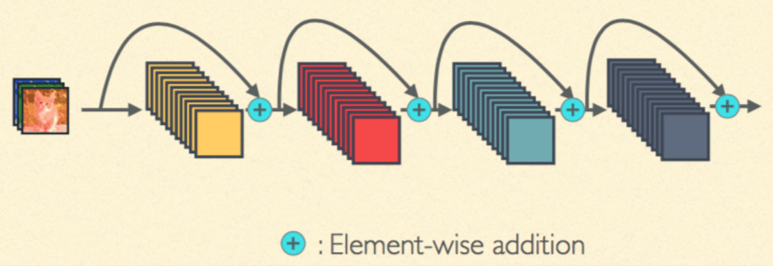
第一张图是 ResNet，第二张图是 DenseNet，因为是在通道维度进行特征的拼接，所以底层的输出会保留进入所有后面的层，这能够更好的保证梯度的传播，同时能够使用低维的特征和高维的特征进行联合训练，能够得到更好的结果。

DenseNet 主要由 dense block 构成，下面我们来实现一个 densen block

import sys
sys.path.append('..')

import numpy as np
import torch
from torch import nn
from torch.autograd import Variable
from torchvision.datasets import CIFAR10

首先定义一个卷积块，这个卷积块的顺序是 bn -> relu -> conv

def conv_block(in_channel, out_channel):
    layer = nn.Sequential(
        nn.BatchNorm2d(in_channel),
        nn.ReLU(True),
        nn.Conv2d(in_channel, out_channel, 3, padding=1, bias=False)
    )
    return layer

dense block 将每次的卷积的输出称为 growth_rate，因为如果输入是 in_channel，有 n 层，那么输出就是 in_channel + n * growh_rate

class dense_block(nn.Module):
    def __init__(self, in_channel, growth_rate, num_layers):
        super(dense_block, self).__init__()
        block = []
        channel = in_channel
        for i in range(num_layers):
            block.append(conv_block(channel, growth_rate))
            channel += growth_rate

        self.net = nn.Sequential(*block)

    def forward(self, x):
        for layer in self.net:
            out = layer(x)
            x = torch.cat((out, x), dim=1)
        return x

我们验证一下输出的 channel 是否正确

test_net = dense_block(3, 12, 3)
test_x = Variable(torch.zeros(1, 3, 96, 96))
print('input shape: {} x {} x {}'.format(test_x.shape[1], test_x.shape[2], test_x.shape[3]))
test_y = test_net(test_x)
print('output shape: {} x {} x {}'.format(test_y.shape[1], test_y.shape[2], test_y.shape[3]))

input shape: 3 x 96 x 96
output shape: 39 x 96 x 96

除了 dense block，DenseNet 中还有一个模块叫过渡层（transition block），因为 DenseNet 会不断地对维度进行拼接， 所以当层数很高的时候，输出的通道数就会越来越大，参数和计算量也会越来越大，为了避免这个问题，需要引入过渡层将输出通道降低下来，同时也将输入的长宽减半，这个过渡层可以使用 1 x 1 的卷积

def transition(in_channel, out_channel):
    trans_layer = nn.Sequential(
        nn.BatchNorm2d(in_channel),
        nn.ReLU(True),
        nn.Conv2d(in_channel, out_channel, 1),
        nn.AvgPool2d(2, 2)
    )
    return trans_layer

验证一下过渡层是否正确

test_net = transition(3, 12)
test_x = Variable(torch.zeros(1, 3, 96, 96))
print('input shape: {} x {} x {}'.format(test_x.shape[1], test_x.shape[2], test_x.shape[3]))
test_y = test_net(test_x)
print('output shape: {} x {} x {}'.format(test_y.shape[1], test_y.shape[2], test_y.shape[3]))

input shape: 3 x 96 x 96
output shape: 12 x 48 x 48

最后我们定义 DenseNet

class densenet(nn.Module):
    def __init__(self, in_channel, num_classes, growth_rate=32, block_layers=[6, 12, 24, 16]):
        super(densenet, self).__init__()
        self.block1 = nn.Sequential(
            nn.Conv2d(in_channel, 64, 7, 2, 3),
            nn.BatchNorm2d(64),
            nn.ReLU(True),
            nn.MaxPool2d(3, 2, padding=1)
        )

        channels = 64
        block = []
        for i, layers in enumerate(block_layers):
            block.append(dense_block(channels, growth_rate, layers))
            channels += layers * growth_rate
            if i != len(block_layers) - 1:
                block.append(transition(channels, channels // 2)) # 通过 transition 层将大小减半，通道数减半
                channels = channels // 2

        self.block2 = nn.Sequential(*block)
        self.block2.add_module('bn', nn.BatchNorm2d(channels))
        self.block2.add_module('relu', nn.ReLU(True))
        self.block2.add_module('avg_pool', nn.AvgPool2d(3))

        self.classifier = nn.Linear(channels, num_classes)

    def forward(self, x):
        x = self.block1(x)
        x = self.block2(x)

        x = x.view(x.shape[0], -1)
        x = self.classifier(x)
        return x

test_net = densenet(3, 10)
test_x = Variable(torch.zeros(1, 3, 96, 96))
test_y = test_net(test_x)
print('output: {}'.format(test_y.shape))

output: torch.Size([1, 10])

from utils import train

def data_tf(x):
    x = x.resize((96, 96), 2) # 将图片放大到 96 x 96
    x = np.array(x, dtype='float32') / 255
    x = (x - 0.5) / 0.5 # 标准化，这个技巧之后会讲到
    x = x.transpose((2, 0, 1)) # 将 channel 放到第一维，只是 pytorch 要求的输入方式
    x = torch.from_numpy(x)
    return x

train_set = CIFAR10('./data', train=True, transform=data_tf)
train_data = torch.utils.data.DataLoader(train_set, batch_size=64, shuffle=True)
test_set = CIFAR10('./data', train=False, transform=data_tf)
test_data = torch.utils.data.DataLoader(test_set, batch_size=128, shuffle=False)

net = densenet(3, 10)
optimizer = torch.optim.SGD(net.parameters(), lr=0.01)
criterion = nn.CrossEntropyLoss()

train(net, train_data, test_data, 20, optimizer, criterion)

Epoch 0. Train Loss: 1.374316, Train Acc: 0.507972, Valid Loss: 1.203217, Valid Acc: 0.572884, Time 00:01:44
Epoch 1. Train Loss: 0.912924, Train Acc: 0.681506, Valid Loss: 1.555908, Valid Acc: 0.492286, Time 00:01:50
Epoch 2. Train Loss: 0.701387, Train Acc: 0.755794, Valid Loss: 0.815147, Valid Acc: 0.718354, Time 00:01:49
Epoch 3. Train Loss: 0.575985, Train Acc: 0.800911, Valid Loss: 0.696013, Valid Acc: 0.759494, Time 00:01:50
Epoch 4. Train Loss: 0.479812, Train Acc: 0.836957, Valid Loss: 1.013879, Valid Acc: 0.676226, Time 00:01:51
Epoch 5. Train Loss: 0.402165, Train Acc: 0.861413, Valid Loss: 0.674512, Valid Acc: 0.778481, Time 00:01:50
Epoch 6. Train Loss: 0.334593, Train Acc: 0.888247, Valid Loss: 0.647112, Valid Acc: 0.791634, Time 00:01:50
Epoch 7. Train Loss: 0.278181, Train Acc: 0.907149, Valid Loss: 0.773517, Valid Acc: 0.756527, Time 00:01:51
Epoch 8. Train Loss: 0.227948, Train Acc: 0.922714, Valid Loss: 0.654399, Valid Acc: 0.800237, Time 00:01:49
Epoch 9. Train Loss: 0.181156, Train Acc: 0.940157, Valid Loss: 1.179013, Valid Acc: 0.685225, Time 00:01:50
Epoch 10. Train Loss: 0.151305, Train Acc: 0.950208, Valid Loss: 0.630000, Valid Acc: 0.807951, Time 00:01:50
Epoch 11. Train Loss: 0.118433, Train Acc: 0.961077, Valid Loss: 1.247253, Valid Acc: 0.703323, Time 00:01:52
Epoch 12. Train Loss: 0.094127, Train Acc: 0.969789, Valid Loss: 1.230697, Valid Acc: 0.723101, Time 00:01:51
Epoch 13. Train Loss: 0.086181, Train Acc: 0.972047, Valid Loss: 0.904135, Valid Acc: 0.769284, Time 00:01:50
Epoch 14. Train Loss: 0.064248, Train Acc: 0.980359, Valid Loss: 1.665002, Valid Acc: 0.624209, Time 00:01:51
Epoch 15. Train Loss: 0.054932, Train Acc: 0.982996, Valid Loss: 0.927216, Valid Acc: 0.774723, Time 00:01:51
Epoch 16. Train Loss: 0.043503, Train Acc: 0.987272, Valid Loss: 1.574383, Valid Acc: 0.707377, Time 00:01:52
Epoch 17. Train Loss: 0.047615, Train Acc: 0.985154, Valid Loss: 0.987781, Valid Acc: 0.770471, Time 00:01:51
Epoch 18. Train Loss: 0.039813, Train Acc: 0.988012, Valid Loss: 2.248944, Valid Acc: 0.631824, Time 00:01:50
Epoch 19. Train Loss: 0.030183, Train Acc: 0.991168, Valid Loss: 0.887785, Valid Acc: 0.795392, Time 00:01:51

DenseNet 将残差连接改为了特征拼接，使得网络有了更稠密的连接