十三、树和森林
作者:Chris Albon
译者:飞龙
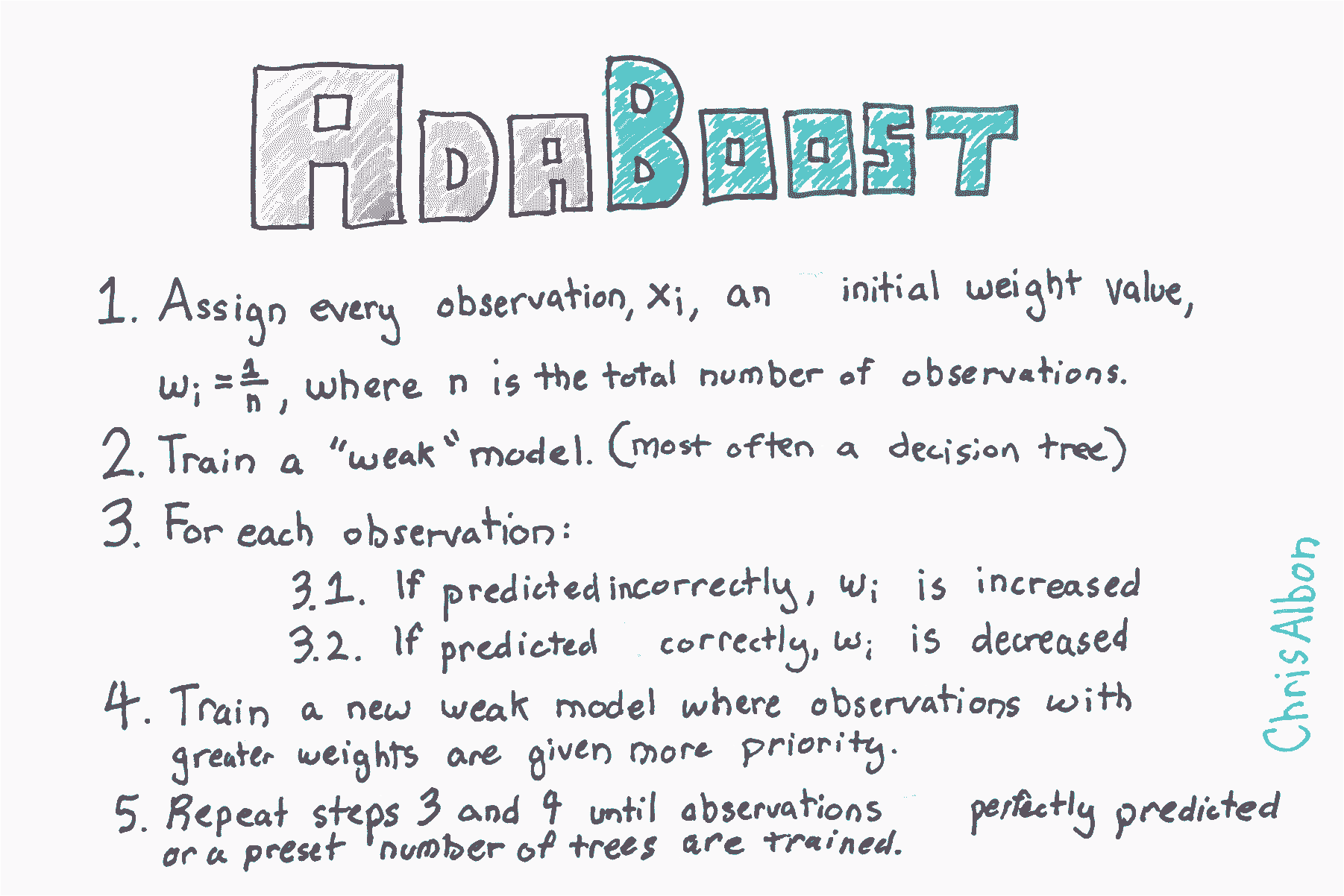
Adaboost 分类器
# 加载库
from sklearn.ensemble import AdaBoostClassifier
from sklearn import datasets

# 加载数据
iris = datasets.load_iris()
X = iris.data
y = iris.target
最重要的参数是base_estimator,n_estimators和learning_rate。
base_estimator是用于训练弱模型的学习算法。 这几乎总是不需要改变,因为到目前为止,与 AdaBoost 一起使用的最常见的学习者是决策树 - 这个参数的默认参数。n_estimators是迭代式训练的模型数。learning_rate是每个模型对权重的贡献,默认为1。 降低学习率将意味着权重将增加或减少到很小的程度,迫使模型训练更慢(但有时会产生更好的表现得分)。loss是AdaBoostRegressor独有的,它设置了更新权重时使用的损失函数。 这默认为线性损失函数,但可以更改为square或exponential。
# 创建 adaboost 决策树分类器对象
clf = AdaBoostClassifier(n_estimators=50,
                         learning_rate=1,
                         random_state=0)

# 训练模型
model = clf.fit(X, y)
决策树分类器
# 加载库
from sklearn.tree import DecisionTreeClassifier
from sklearn import datasets
# 加载数据
iris = datasets.load_iris()
X = iris.data
y = iris.target
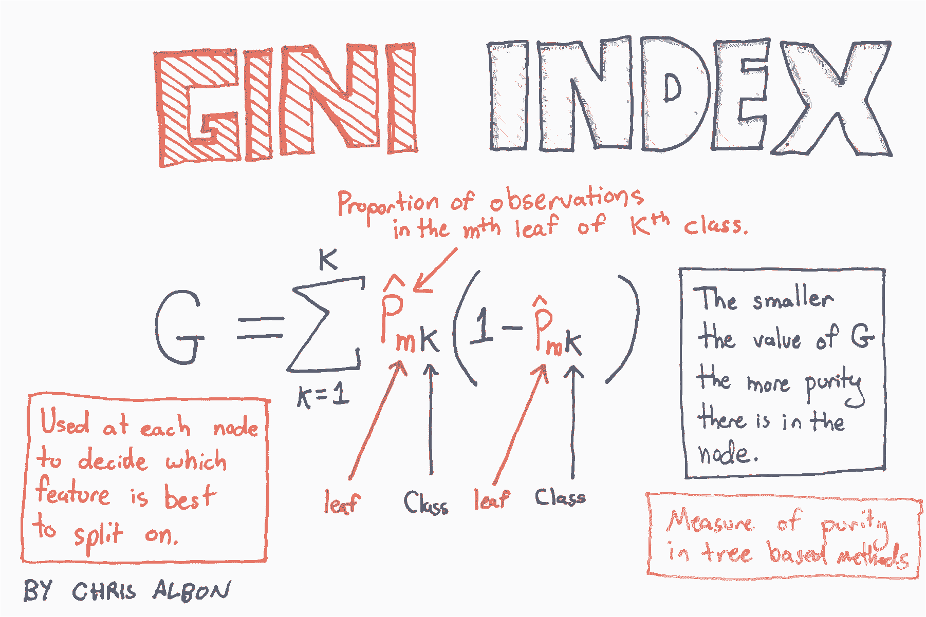
# 创建使用 GINI 的决策树分类器对象
clf = DecisionTreeClassifier(criterion='gini', random_state=0)
# 训练模型
model = clf.fit(X, y)
# 生成新的观测
observation = [[ 5, 4, 3, 2]]
# 预测观测的类别
model.predict(observation)
# array([1])
# 查看三个类别的预测概率
model.predict_proba(observation)
# array([[ 0., 1., 0.]])
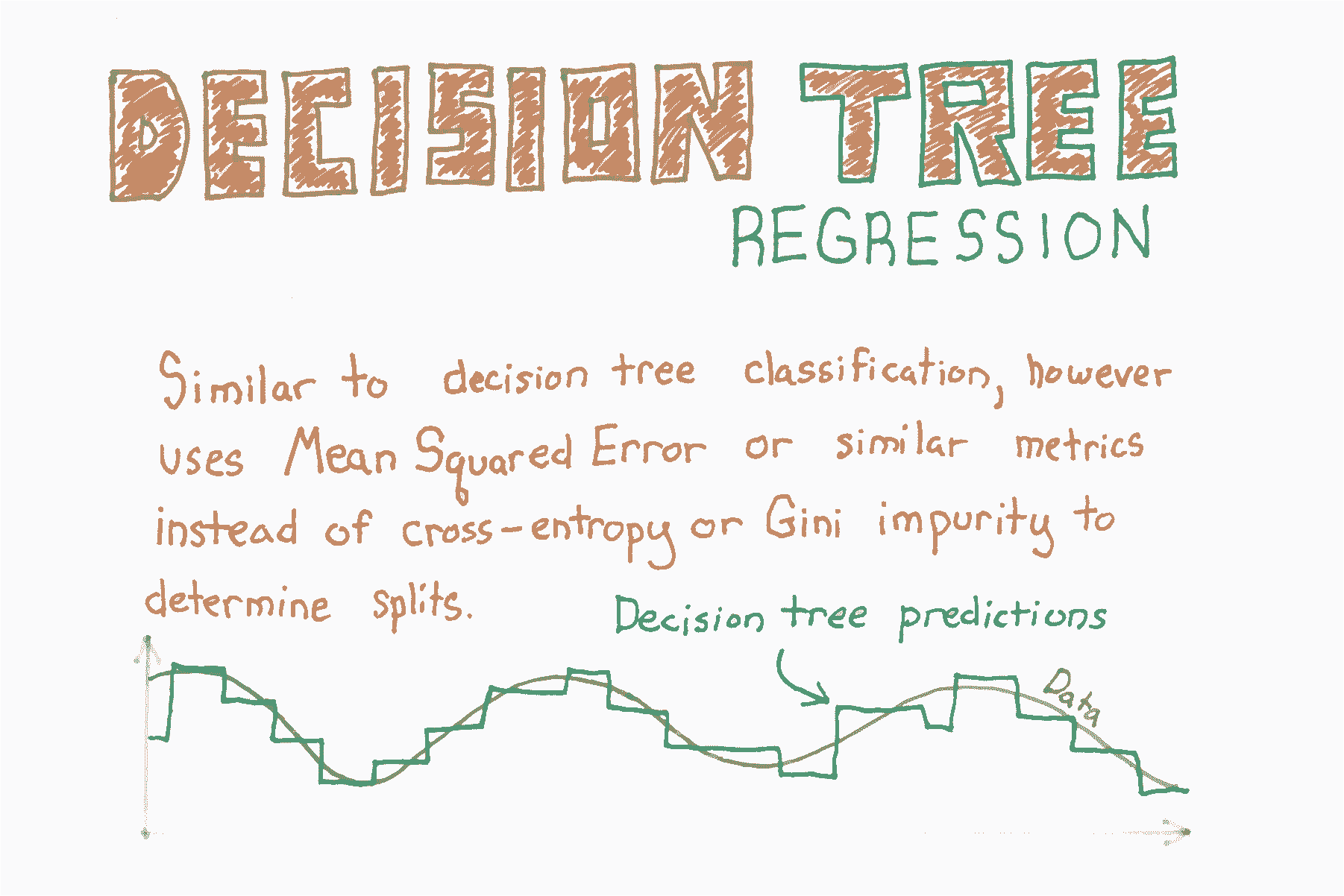
决策树回归
# 加载库
from sklearn.tree import DecisionTreeRegressor
from sklearn import datasets

# 加载只有两个特征的数据
boston = datasets.load_boston()
X = boston.data[:,0:2]
y = boston.target
决策树回归的工作方式类似于决策树分类,但不是减少基尼杂质或熵,而是测量潜在的分割点,它们减少均方误差(MSE)的程度:
其中  是目标的真实值,
 是预测值。
是预测值。
# 创建决策树回归器对象
regr = DecisionTreeRegressor(random_state=0)

# 训练模型
model = regr.fit(X, y)

# 生成新的观测
observation = [[0.02, 16]]

# 预测观测的值
model.predict(observation)

# array([ 33.])
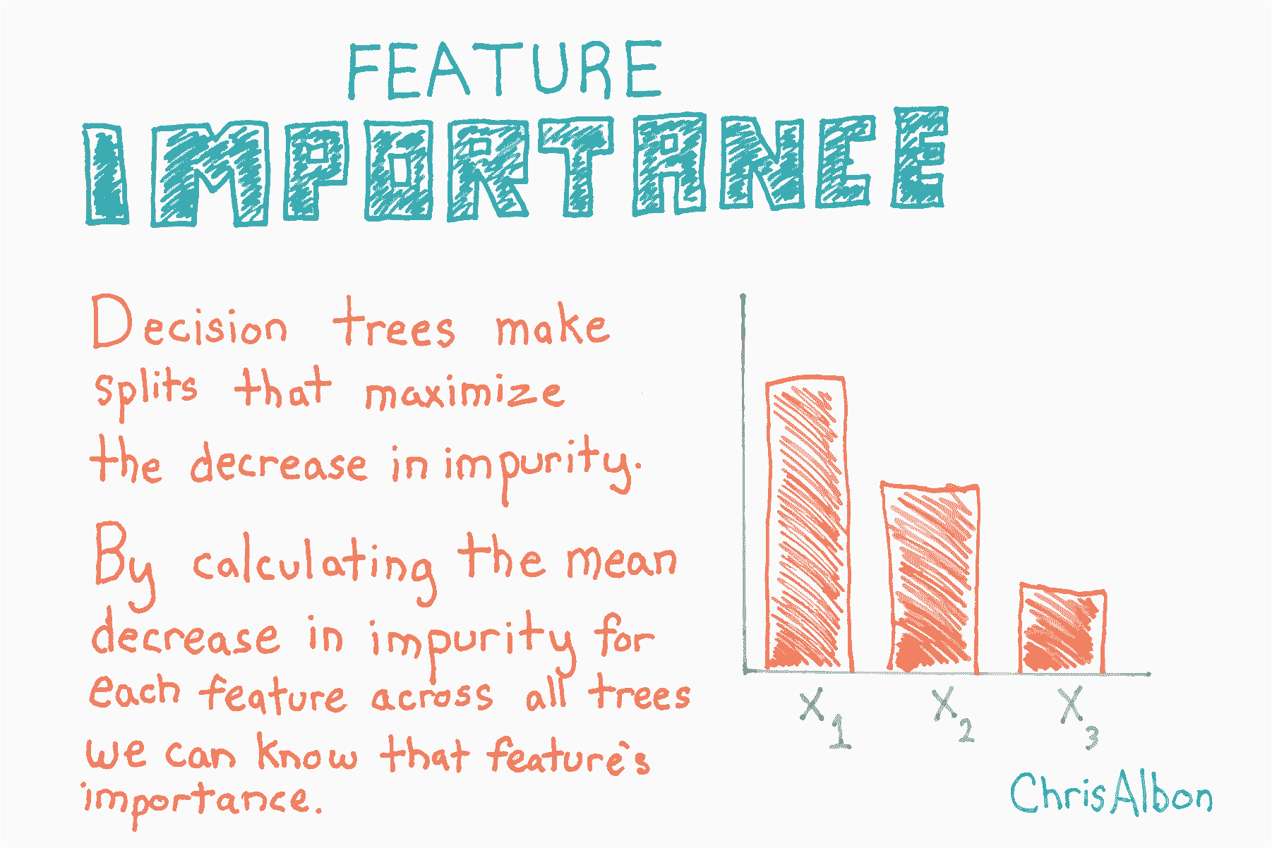
特征的重要性
# 加载库
from sklearn.ensemble import RandomForestClassifier
from sklearn import datasets
import numpy as np
import matplotlib.pyplot as plt

# 加载数据
iris = datasets.load_iris()
X = iris.data
y = iris.target

# 创建决策树分类器对象
clf = RandomForestClassifier(random_state=0, n_jobs=-1)

# 训练模型
model = clf.fit(X, y)

# 计算特征重要性
importances = model.feature_importances_

# 对特征重要性降序排序
indices = np.argsort(importances)[::-1]

# 重新排列特征名称,使它们匹配有序的特征重要性
names = [iris.feature_names[i] for i in indices]

# 创建绘图
plt.figure()

# 创建绘图标题
plt.title("Feature Importance")

# 添加条形
plt.bar(range(X.shape[1]), importances[indices])

# 添加特征名称作为 x 轴标签
plt.xticks(range(X.shape[1]), names, rotation=90)

# 展示绘图
plt.show()

使用随机森林的特征选择
通常在数据科学中,我们有数百甚至数百万个特征,我们想要一种方法来创建仅包含最重要特征的模型。 这有三个好处。 首先,我们使模型更易于解释。 其次,我们可以减少模型的方差,从而避免过拟合。 最后,我们可以减少训练模型的计算开销(和时间)。 仅识别最相关特征的过程称为“特征选择”。
数据科学工作流程中,随机森林通常用于特征选择。 原因是,随机森林使用的基于树的策略,自然按照它们如何改善节点的纯度来排序。 这意味着所有树的不纯度的减少(称为基尼不纯度)。 不纯度减少最多的节点出现在树的开始处,而不纯度减少最少的节点出现在树的末端。 因此,通过在特定节点下修剪树,我们可以创建最重要特征的子集。
在这个教程中,我们将要:
- 准备数据集
- 训练随机森林分类器
- 识别最重要的特征
- 创建新的“有限特征的”数据集,仅仅包含那些特征
- 在新数据集上训练第二个分类器
- 将“全部特征的”分类器的准确率,和“有限特征的”分类器比较
注:还有其他重要定义,但在本教程中,我们将讨论限制为基尼重要性。
import numpy as np
from sklearn.ensemble import RandomForestClassifier
from sklearn import datasets
from sklearn.model_selection import train_test_split
from sklearn.feature_selection import SelectFromModel
from sklearn.metrics import accuracy_score
本教程中使用的数据集是着名的鸢尾花数据集鸢尾花数据包含来自三种鸢尾y和四个特征变量X的 50 个样本。
# 加载鸢尾花数据集
iris = datasets.load_iris()

# 创建特征名称列表
feat_labels = ['Sepal Length','Sepal Width','Petal Length','Petal Width']

# 从特征中创建 X
X = iris.data

# 从目标中创建 y
y = iris.target

# 查看特征
X[0:5]

'''
array([[ 5.1,  3.5,  1.4,  0.2],
       [ 4.9,  3\. ,  1.4,  0.2],
       [ 4.7,  3.2,  1.3,  0.2],
       [ 4.6,  3.1,  1.5,  0.2],
       [ 5\. ,  3.6,  1.4,  0.2]])
'''

# 查看目标数据
y

'''
array([0, 0, 0, 0, 0, 0, 0, 0, 0, 0, 0, 0, 0, 0, 0, 0, 0, 0, 0, 0, 0, 0, 0,
       0, 0, 0, 0, 0, 0, 0, 0, 0, 0, 0, 0, 0, 0, 0, 0, 0, 0, 0, 0, 0, 0, 0,
       0, 0, 0, 0, 1, 1, 1, 1, 1, 1, 1, 1, 1, 1, 1, 1, 1, 1, 1, 1, 1, 1, 1,
       1, 1, 1, 1, 1, 1, 1, 1, 1, 1, 1, 1, 1, 1, 1, 1, 1, 1, 1, 1, 1, 1, 1,
       1, 1, 1, 1, 1, 1, 1, 1, 2, 2, 2, 2, 2, 2, 2, 2, 2, 2, 2, 2, 2, 2, 2,
       2, 2, 2, 2, 2, 2, 2, 2, 2, 2, 2, 2, 2, 2, 2, 2, 2, 2, 2, 2, 2, 2, 2,
       2, 2, 2, 2, 2, 2, 2, 2, 2, 2, 2, 2])
'''

# 将数据分为 40% 的测试和 60% 的训练集
X_train, X_test, y_train, y_test = train_test_split(X, y, test_size=0.4, random_state=0)

# 创建随机森林分类器
clf = RandomForestClassifier(n_estimators=10000, random_state=0, n_jobs=-1)

# 训练分类器
clf.fit(X_train, y_train)

# 打印每个特征的名称和基尼重要性
for feature in zip(feat_labels, clf.feature_importances_):
    print(feature)

'''
('Sepal Length', 0.11024282328064565)
('Sepal Width', 0.016255033655398394)
('Petal Length', 0.45028123999239533)
('Petal Width', 0.42322090307156124)
'''
上面的得分是每个变量的重要性得分。 有两点需要注意。 首先,所有重要性得分加起来为 100%。 其次,“花瓣长度”和“花瓣宽度”远比其他两个特征重要。结合起来,“花瓣长度”和“花瓣宽度”的重要性约为 0.86!显然,这些是最重要的特征。
# 创建一个选择器对象,
# 该对象将使用随机森林分类器来标识重要性大于 0.15 的特征
sfm = SelectFromModel(clf, threshold=0.15)

# 训练选择器
sfm.fit(X_train, y_train)

'''
SelectFromModel(estimator=RandomForestClassifier(bootstrap=True, class_weight=None, criterion='gini',
            max_depth=None, max_features='auto', max_leaf_nodes=None,
            min_impurity_split=1e-07, min_samples_leaf=1,
            min_samples_split=2, min_weight_fraction_leaf=0.0,
            n_estimators=10000, n_jobs=-1, oob_score=False, random_state=0,
            verbose=0, warm_start=False),
        prefit=False, threshold=0.15)
'''

# 打印最重要的特征的名称
for feature_list_index in sfm.get_support(indices=True):
    print(feat_labels[feature_list_index])

'''
Petal Length
Petal Width
'''

# 转换数据来创建仅包含最重要特征的新数据集
# 注意:我们必须将变换应用于训练 X 和测试 X 数据。
X_important_train = sfm.transform(X_train)
X_important_test = sfm.transform(X_test)

# 为最重要的特征创建新的随机森林分类器
clf_important = RandomForestClassifier(n_estimators=10000, random_state=0, n_jobs=-1)

# 在包含最重要特征的新数据集上训练新分类器
clf_important.fit(X_important_train, y_train)

'''
RandomForestClassifier(bootstrap=True, class_weight=None, criterion='gini',
            max_depth=None, max_features='auto', max_leaf_nodes=None,
            min_impurity_split=1e-07, min_samples_leaf=1,
            min_samples_split=2, min_weight_fraction_leaf=0.0,
            n_estimators=10000, n_jobs=-1, oob_score=False, random_state=0,
            verbose=0, warm_start=False)
'''

# 将全部特征的分类器应用于测试数据
y_pred = clf.predict(X_test)

# 查看我们的全部特征(4 个特征)的模型的准确率
accuracy_score(y_test, y_pred)

# 0.93333333333333335

# 将全部特征的分类器应用于测试数据
y_important_pred = clf_important.predict(X_important_test)

# 查看我们有限特征(2 个特征)的模型的准确率
accuracy_score(y_test, y_important_pred)

# 0.8833333333333333
从准确率得分可以看出,包含所有四个特征的原始模型准确率为 93.3%,而仅包含两个特征的“有限”模型准确率为 88.3%。 因此,为了精确率的低成本,我们将模型中的特征数量减半。
在随机森林中处理不平衡类别
# 加载库
from sklearn.ensemble import RandomForestClassifier
import numpy as np
from sklearn import datasets

# 加载数据
iris = datasets.load_iris()
X = iris.data
y = iris.target

# 通过移除前 40 个观测,生成高度不平衡的类别
X = X[40:,:]
y = y[40:]

# 创建目标向量,表示类别是否为 0
y = np.where((y == 0), 0, 1)
当使用RandomForestClassifier时,有用的设置是class_weight = balanced,其中类自动加权,与它们在数据中出现的频率成反比。具体来说:

其中  是类
是类  的权重,
的权重, 是观测数,
是观测数, 是类 中的观测数,
 是类的总数。
# 创建决策树分类器对象
clf = RandomForestClassifier(random_state=0, n_jobs=-1, class_weight="balanced")

# 训练模型
model = clf.fit(X, y)
随机森林分类器
# 加载库
from sklearn.ensemble import RandomForestClassifier
from sklearn import datasets

# 加载数据
iris = datasets.load_iris()
X = iris.data
y = iris.target

# 创建使用熵的随机森林分类器
clf = RandomForestClassifier(criterion='entropy', random_state=0, n_jobs=-1)

# 训练模型
model = clf.fit(X, y)

# 创建新的观测
observation = [[ 5,  4,  3,  2]]

# 预测观测的类别
model.predict(observation)
array([1])
随机森林分类器示例
本教程基于 Yhat 2013 年的[ Python 中的随机森林]教程(http://blog.yhat.com/posts/random-forests-in-python.html)。 如果你想要随机森林的理论和用途的总结,我建议你查看他们的指南。 在下面的教程中,我对文章末尾提供的随机森林的简短代码示例进行了注释,更正和扩展。 具体来说,我(1)更新代码,使其在最新版本的 pandas 和 Python 中运行,(2)编写详细的注释,解释每个步骤中发生的事情,以及(3)以多种方式扩展代码。
让我们开始吧!
数据的注解
本教程的数据很有名。 被称为鸢尾花数据集,它包含四个变量,测量了三个鸢尾花物种的各个部分,然后是带有物种名称的第四个变量。 它在机器学习和统计社区中如此着名的原因是,数据需要很少的预处理(即没有缺失值,所有特征都是浮点数等)。
# 加载鸢尾花数据集
from sklearn.datasets import load_iris

# 加载 sklearn 的随机森林分类器
from sklearn.ensemble import RandomForestClassifier

# 加载 pandas
import pandas as pd

# 加载 numpy
import numpy as np

# 设置随机种子
np.random.seed(0)

# Create an object called iris with the iris data
iris = load_iris()

# 创建带有四个特征变量的数据帧
df = pd.DataFrame(iris.data, columns=iris.feature_names)

# 查看前五行
df.head()
| sepal length (cm) | sepal width (cm) | petal length (cm) | petal width (cm) | |
|---|---|---|---|---|
| 0 | 5.1 | 3.5 | 1.4 | 0.2 |
| 1 | 4.9 | 3.0 | 1.4 | 0.2 |
| 2 | 4.7 | 3.2 | 1.3 | 0.2 |
| 3 | 4.6 | 3.1 | 1.5 | 0.2 |
| 4 | 5.0 | 3.6 | 1.4 | 0.2 |
# 添加带有物种名称的新列,我们要尝试预测它
df['species'] = pd.Categorical.from_codes(iris.target, iris.target_names)

# 查看前五行
df.head()
| sepal length (cm) | sepal width (cm) | petal length (cm) | petal width (cm) | species | |
|---|---|---|---|---|---|
| 0 | 5.1 | 3.5 | 1.4 | 0.2 | setosa |
| 1 | 4.9 | 3.0 | 1.4 | 0.2 | setosa |
| 2 | 4.7 | 3.2 | 1.3 | 0.2 | setosa |
| 3 | 4.6 | 3.1 | 1.5 | 0.2 | setosa |
| 4 | 5.0 | 3.6 | 1.4 | 0.2 | setosa |
# 创建一个新列,每列生成一个0到1之间的随机数,
# 如果该值小于或等于.75,则将该单元格的值设置为 True
# 否则为 False。这是一种简洁方式,
# 随机分配一些行作为训练数据,一些作为测试数据。
df['is_train'] = np.random.uniform(0, 1, len(df)) <= .75

# 查看前五行
df.head()
| sepal length (cm) | sepal width (cm) | petal length (cm) | petal width (cm) | species | is_train | |
|---|---|---|---|---|---|---|
| 0 | 5.1 | 3.5 | 1.4 | 0.2 | setosa | True |
| 1 | 4.9 | 3.0 | 1.4 | 0.2 | setosa | True |
| 2 | 4.7 | 3.2 | 1.3 | 0.2 | setosa | True |
| 3 | 4.6 | 3.1 | 1.5 | 0.2 | setosa | True |
| 4 | 5.0 | 3.6 | 1.4 | 0.2 | setosa | True |
# 创建两个新的数据帧,一个包含训练行,另一个包含测试行
train, test = df[df['is_train']==True], df[df['is_train']==False]

# 显示测试和训练数据帧的观测数
print('Number of observations in the training data:', len(train))
print('Number of observations in the test data:',len(test))

'''
Number of observations in the training data: 118
Number of observations in the test data: 32
'''

# 创建特征列名称的列表
features = df.columns[:4]

# 查看特征
features

'''
Index(['sepal length (cm)', 'sepal width (cm)', 'petal length (cm)',
       'petal width (cm)'],
      dtype='object')
'''

# train['species'] 包含实际的物种名称。
# 在我们使用它之前,我们需要将每个物种名称转换为数字。
# 因此,在这种情况下,有三种物种,它们被编码为 0, 1 或 2。
y = pd.factorize(train['species'])[0]

# 查看目标
y

'''
array([0, 0, 0, 0, 0, 0, 0, 0, 0, 0, 0, 0, 0, 0, 0, 0, 0, 0, 0, 0, 0, 0, 0,
       0, 0, 0, 0, 0, 0, 0, 0, 0, 0, 0, 0, 0, 0, 1, 1, 1, 1, 1, 1, 1, 1, 1,
       1, 1, 1, 1, 1, 1, 1, 1, 1, 1, 1, 1, 1, 1, 1, 1, 1, 1, 1, 1, 1, 1, 1,
       1, 1, 1, 1, 1, 1, 1, 1, 1, 1, 1, 2, 2, 2, 2, 2, 2, 2, 2, 2, 2, 2, 2,
       2, 2, 2, 2, 2, 2, 2, 2, 2, 2, 2, 2, 2, 2, 2, 2, 2, 2, 2, 2, 2, 2, 2,
       2, 2, 2])
'''

# 创建随机森林分类器。按照惯例,clf 表示“分类器”
clf = RandomForestClassifier(n_jobs=2, random_state=0)

# 训练分类器,来接受训练特征
# 并了解它们与训练集 y(物种)的关系
clf.fit(train[features], y)

'''
RandomForestClassifier(bootstrap=True, class_weight=None, criterion='gini',
            max_depth=None, max_features='auto', max_leaf_nodes=None,
            min_impurity_split=1e-07, min_samples_leaf=1,
            min_samples_split=2, min_weight_fraction_leaf=0.0,
            n_estimators=10, n_jobs=2, oob_score=False, random_state=0,
            verbose=0, warm_start=False)
'''
好哇! 我们做到了! 我们正式训练了我们的随机森林分类器! 现在让我们玩玩吧。 分类器模型本身存储在clf变量中。
如果你一直跟着,你会知道我们只在部分数据上训练了我们的分类器,留出了剩下的数据。 在我看来,这是机器学习中最重要的部分。 为什么? 因为省略了部分数据,我们有一组数据来测试我们模型的准确率!
让我们现在实现它。
# 将我们训练的分类器应用于测试数据
# (记住,以前从未见过它)
clf.predict(test[features])

'''
array([0, 0, 0, 0, 0, 0, 0, 0, 0, 0, 0, 0, 0, 1, 1, 1, 2, 2, 1, 1, 2, 2, 2,
       2, 2, 2, 2, 2, 2, 2, 2, 2])
'''
你在上面看到什么? 请记住,我们将三种植物中的每一种编码为 0, 1 或 2。 以上数字列表显示,我们的模型基于萼片长度,萼片宽度,花瓣长度和花瓣宽度,预测每种植物的种类。 分类器对于每种植物有多自信? 我们也可以看到。
# 查看前 10 个观测值的预测概率
clf.predict_proba(test[features])[0:10]

'''
array([[ 1\. ,  0\. ,  0\. ],
       [ 1\. ,  0\. ,  0\. ],
       [ 1\. ,  0\. ,  0\. ],
       [ 1\. ,  0\. ,  0\. ],
       [ 1\. ,  0\. ,  0\. ],
       [ 1\. ,  0\. ,  0\. ],
       [ 1\. ,  0\. ,  0\. ],
       [ 0.9,  0.1,  0\. ],
       [ 1\. ,  0\. ,  0\. ],
       [ 1\. ,  0\. ,  0\. ]])
'''
有三种植物,因此[1, 0, 0]告诉我们分类器确定植物是第一类。 再举一个例子,[0.9, 0.1, 0]告诉我们,分类器给出植物属于第一类的概率为90%,植物属于第二类的概率为 10%。 因为 90 大于 10,分类器预测植物是第一类。
现在我们已经预测了测试数据中所有植物的种类,我们可以比较我们预测的物种与该植物的实际物种。
# 为每个预测的植物类别
# 创建植物的实际英文名称
preds = iris.target_names[clf.predict(test[features])]

# 查看前五个观测值的预测物种
preds[0:5]

'''
array(['setosa', 'setosa', 'setosa', 'setosa', 'setosa'],
      dtype='<U10')
'''

# 查看前五个观测值的实际物种
test['species'].head()

'''
7     setosa
8     setosa
10    setosa
13    setosa
17    setosa
Name: species, dtype: category
Categories (3, object): [setosa, versicolor, virginica]
'''
看起来很不错! 至少对于前五个观测。 现在让我们看看所有数据。
混淆矩阵可能令人混淆,但它实际上非常简单。 列是我们为测试数据预测的物种,行是测试数据的实际物种。 因此,如果我们选取最上面的行,我们可以完美地预测测试数据中的所有 13 个山鸢尾。 然而,在下一行中,我们正确地预测了 5 个杂色鸢尾,但错误地将两个杂色鸢尾预测为维吉尼亚鸢尾。
混淆矩阵的简短解释方式是:对角线上的任何东西都被正确分类,对角线之外的任何东西都被错误地分类。
# 创建混淆矩阵
pd.crosstab(test['species'], preds, rownames=['Actual Species'], colnames=['Predicted Species'])
| Predicted Species | setosa | versicolor | virginica |
|---|---|---|---|
| Actual Species | |||
| setosa | 13 | 0 | 0 |
| versicolor | 0 | 5 | 2 |
| virginica | 0 | 0 | 12 |
虽然我们没有像 OLS 那样得到回归系数,但我们得到的分数告诉我们,每个特征在分类中的重要性。 这是随机森林中最强大的部分之一,因为我们可以清楚地看到,在分类中花瓣宽度比萼片宽度更重要。
# 查看特征列表和它们的重要性得分
list(zip(train[features], clf.feature_importances_))

'''
[('sepal length (cm)', 0.11185992930506346),
 ('sepal width (cm)', 0.016341813006098178),
 ('petal length (cm)', 0.36439533040889194),
 ('petal width (cm)', 0.5074029272799464)]
'''
随机森林回归
# 加载库
from sklearn.ensemble import RandomForestRegressor
from sklearn import datasets

# 加载只有两个特征的数据
boston = datasets.load_boston()
X = boston.data[:,0:2]
y = boston.target

# Create decision tree classifer object
regr = RandomForestRegressor(random_state=0, n_jobs=-1)

# 训练模型
model = regr.fit(X, y)
在随机森林中选择特征重要性
# 加载库
from sklearn.ensemble import RandomForestClassifier
from sklearn import datasets
from sklearn.feature_selection import SelectFromModel

# 加载数据
iris = datasets.load_iris()
X = iris.data
y = iris.target

# 创建随机森林分类器
clf = RandomForestClassifier(random_state=0, n_jobs=-1)
数字越大,特征越重要(所有重要性得分总和为1)。 通过绘制这些值,我们可以为随机森林模型添加可解释性。
# 创建选择重要性大于或等于阈值的特征的对象
selector = SelectFromModel(clf, threshold=0.3)

# 使用选择器生成新的特征矩阵
X_important = selector.fit_transform(X, y)

# 查看特征的前五个观测
X_important[0:5]

'''
array([[ 1.4,  0.2],
       [ 1.4,  0.2],
       [ 1.3,  0.2],
       [ 1.5,  0.2],
       [ 1.4,  0.2]])
'''

# 使用最重要的特征训练随机森林
model = clf.fit(X_important, y)
泰坦尼克比赛和随机森林
import pandas as pd
import numpy as np
from sklearn import preprocessing
from sklearn.ensemble import RandomForestClassifier
from sklearn.model_selection import GridSearchCV, cross_val_score
import csv as csv
你可以在 Kaggle 获取数据。
# 加载数据
train = pd.read_csv('data/train.csv')
test = pd.read_csv('data/test.csv')

# 创建特征列表,我们最终会接受他们
features = ['Age', 'SibSp','Parch','Fare','male','embarked_Q','embarked_S','Pclass_2', 'Pclass_3']
性别
在这里,我们将性别标签(male,female)转换为虚拟变量(1,0)。
# 创建编码器
sex_encoder = preprocessing.LabelEncoder()

# 使编码器拟合训练数据,因此它知道 male = 1
sex_encoder.fit(train['Sex'])

# 将编码器应用于训练数据
train['male'] = sex_encoder.transform(train['Sex'])

# 将编码器应用于测试数据
test['male'] = sex_encoder.transform(test['Sex'])

# 使用单热编码,将编码的特征转换为虚拟值
# 去掉第一个类别来防止共线性
train_embarked_dummied = pd.get_dummies(train["Embarked"], prefix='embarked', drop_first=True)

# 使用单热编码
# 将“已编码”的测试特征转换为虚拟值
# 去掉第一个类别来防止共线性
test_embarked_dummied = pd.get_dummies(test["Embarked"], prefix='embarked', drop_first=True)

# 将虚拟值的数据帧与主数据帧连接起来
train = pd.concat([train, train_embarked_dummied], axis=1)
test = pd.concat([test, test_embarked_dummied], axis=1)

# 使用单热编码将 Pclass 训练特征转换为虚拟值
# 去掉第一个类别来防止共线性
train_Pclass_dummied = pd.get_dummies(train["Pclass"], prefix='Pclass', drop_first=True)

# 使用单热编码将 Pclass 测试特征转换为虚拟值
# 去掉第一个类别来防止共线性
test_Pclass_dummied = pd.get_dummies(test["Pclass"], prefix='Pclass', drop_first=True)

# 将虚拟值的数据帧与主数据帧连接起来
train = pd.concat([train, train_Pclass_dummied], axis=1)
test = pd.concat([test, test_Pclass_dummied], axis=1)
年龄
Age特征的许多值都缺失,并且会妨碍随机森林进行训练。 我们解决这个问题,我们将用年龄的平均值填充缺失值(一个实用的操作)。
# 创建填充器对象
age_imputer = preprocessing.Imputer(missing_values='NaN', strategy='mean', axis=0)

# 将填充器对象拟合训练数据
age_imputer.fit(train['Age'].reshape(-1, 1))

# 将填充器对象应用于训练和测试数据
train['Age'] = age_imputer.transform(train['Age'].reshape(-1, 1))
test['Age'] = age_imputer.transform(test['Age'].reshape(-1, 1))

# 创建填充器对象
fare_imputer = preprocessing.Imputer(missing_values='NaN', strategy='mean', axis=0)

# 将填充器对象拟合训练数据
fare_imputer.fit(train['Fare'].reshape(-1, 1))

# 将填充器对象应用于训练和测试数据
train['Fare'] = fare_imputer.transform(train['Fare'].reshape(-1, 1))
test['Fare'] = fare_imputer.transform(test['Fare'].reshape(-1, 1))

# 创建包含参数所有候选值的字典
parameter_grid = dict(n_estimators=list(range(1, 5001, 1000)),
                      criterion=['gini','entropy'],
                      max_features=list(range(1, len(features), 2)),
                      max_depth= [None] + list(range(5, 25, 1)))

# 创建随机森林对象
random_forest = RandomForestClassifier(random_state=0, n_jobs=-1)

# 创建网格搜索对象,使用 5 倍交叉验证
# 并使用所有核(n_jobs = -1)
clf = GridSearchCV(estimator=random_forest, param_grid=parameter_grid, cv=5, verbose=1, n_jobs=-1)

# 将网格搜索嵌套在 3 折 CV 中来进行模型评估
cv_scores = cross_val_score(clf, train[features], train['Survived'])

# 打印结果
print('Accuracy scores:', cv_scores)
print('Mean of score:', np.mean(cv_scores))
print('Variance of scores:', np.var(cv_scores))

# 在整个数据集上重新训练模型
clf.fit(train[features], train['Survived'])

# 预测在测试数据集中的幸存者
predictions = clf.predict(test[features])

# 获取乘客 ID
ids = test['PassengerId'].values

# 创建 csv
submission_file = open("submission.csv", "w")

# 写入这个 csv
open_file_object = csv.writer(submission_file)

# 写入 CSV 标题
open_file_object.writerow(["PassengerId","Survived"])

# 写入 CSV 的行
open_file_object.writerows(zip(ids, predictions))

# 关闭文件
submission_file.close()
可视化决策树
# 加载库
from sklearn.tree import DecisionTreeClassifier
from sklearn import datasets
from IPython.display import Image
from sklearn import tree
import pydotplus

# 加载数据
iris = datasets.load_iris()
X = iris.data
y = iris.target

# 创建决策树分类器对象
clf = DecisionTreeClassifier(random_state=0)

# 训练模型
model = clf.fit(X, y)

# 创建 DOT 数据
dot_data = tree.export_graphviz(clf, out_file=None,
                                feature_names=iris.feature_names,
                                class_names=iris.target_names)

# 绘制图形
graph = pydotplus.graph_from_dot_data(dot_data)

# 展示图形
Image(graph.create_png())

# 创建 PDF
graph.write_pdf("iris.pdf")

# 创建 PNG
graph.write_png("iris.png")

# True