3.2 Functions and the Processes They Generate

A function is a pattern for the local evolution of a computational process. It specifies how each stage of the process is built upon the previous stage. We would like to be able to make statements about the overall behavior of a process whose local evolution has been specified by one or more functions. This analysis is very difficult to do in general, but we can at least try to describe some typical patterns of process evolution.

In this section we will examine some common "shapes" for processes generated by simple functions. We will also investigate the rates at which these processes consume the important computational resources of time and space.

3.2.1 Recursive Functions

A function is called recursive if the body of that function calls the function itself, either directly or indirectly. That is, the process of executing the body of a recursive function may in turn require applying that function again. Recursive functions do not require any special syntax in Python, but they do require some care to define correctly.

As an introduction to recursive functions, we begin with the task of converting an English word into its Pig Latin equivalent. Pig Latin is a secret language: one that applies a simple, deterministic transformation to each word that veils the meaning of the word. Thomas Jefferson was supposedly an early adopter. The Pig Latin equivalent of an English word moves the initial consonant cluster (which may be empty) from the beginning of the word to the end and follows it by the "-ay" vowel. Hence, the word "pun" becomes "unpay", "stout" becomes "outstay", and "all" becomes "allay".

>>> def pig_latin(w):
        """Return the Pig Latin equivalent of English word w."""
        if starts_with_a_vowel(w):
            return w + 'ay'
        return pig_latin(w[1:] + w[0])

>>> def starts_with_a_vowel(w):
        """Return whether w begins with a vowel."""
        return w[0].lower() in 'aeiou'

The idea behind this definition is that the Pig Latin variant of a string that starts with a consonant is the same as the Pig Latin variant of another string: that which is created by moving the first letter to the end. Hence, the Pig Latin word for "sending" is the same as for "endings" (endingsay), and the Pig Latin word for "smother" is the same as the Pig Latin word for "mothers" (othersmay). Moreover, moving one consonant from the beginning of the word to the end results in a simpler problem with fewer initial consonants. In the case of "sending", moving the "s" to the end gives a word that starts with a vowel, and so our work is done.

This definition of pig_latin is both complete and correct, even though the pig_latin function is called within its own body.

>>> pig_latin('pun')
'unpay'

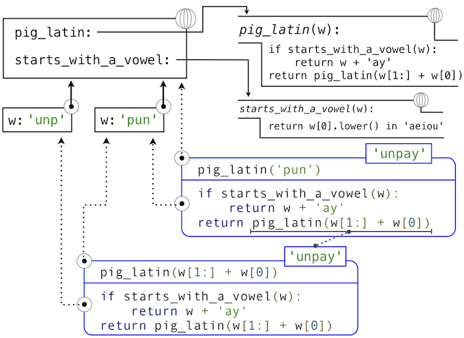
The idea of being able to define a function in terms of itself may be disturbing; it may seem unclear how such a "circular" definition could make sense at all, much less specify a well-defined process to be carried out by a computer. We can, however, understand precisely how this recursive function applies successfully using our environment model of computation. The environment diagram and expression tree that depict the evaluation of pig_latin('pun') appear below.

The steps of the Python evaluation procedures that produce this result are:

1. The def statement for pig_latin is executed, which

> 1. Creates a new pig_latin function object with the stated body, and > 2. Binds the name pig_latin to that function in the current (global) frame

1. The def statement for starts_with_a_vowel is executed similarly
2. The call expression pig_latin('pun') is evaluated by

> 1. Evaluating the operator and operand sub-expressions by > > > 1. Looking up the name pig_latin that is bound to the pig_latin function > > 2. Evaluating the operand string literal to the string object 'pun' > > 1. Applying the function pig_latin to the argument 'pun' by > > > 1. Adding a local frame that extends the global frame > > 2. Binding the formal parameter w to the argument 'pun' in that frame > > 3. Executing the body of pig_latin in the environment that starts with that frame: > > > > > 1. The initial conditional statement has no effect, because the header expression evaluates to False. > > > 2. The final return expression pig_latin(w[1:] + w[0]) is evaluated by > > > > > > > 1. Looking up the name pig_latin that is bound to the pig_latin function > > > > 2. Evaluating the operand expression to the string object 'unp' > > > > 3. Applying pig_latin to the argument 'unp', which returns the desired result from the suite of the conditional statement in the body of pig_latin.

As this example illustrates, a recursive function applies correctly, despite its circular character. The pig_latin function is applied twice, but with a different argument each time. Although the second call comes from the body of pig_latin itself, looking up that function by name succeeds because the name pig_latin is bound in the environment before its body is executed.

This example also illustrates how Python's recursive evaluation procedure can interact with a recursive function to evolve a complex computational process with many nested steps, even though the function definition may itself contain very few lines of code.

3.2.2 The Anatomy of Recursive Functions

A common pattern can be found in the body of many recursive functions. The body begins with a base case, a conditional statement that defines the behavior of the function for the inputs that are simplest to process. In the case of pig_latin, the base case occurs for any argument that starts with a vowel. In this case, there is no work left to be done but return the argument with "ay" added to the end. Some recursive functions will have multiple base cases.

The base cases are then followed by one or more recursive calls. Recursive calls require a certain character: they must simplify the original problem. In the case of pig_latin, the more initial consonants in w, the more work there is left to do. In the recursive call, pig_latin(w[1:] + w[0]), we call pig_latin on a word that has one fewer initial consonant -- a simpler problem. Each successive call to pig_latin will be simpler still until the base case is reached: a word with no initial consonants.

Recursive functions express computation by simplifying problems incrementally. They often operate on problems in a different way than the iterative approaches that we have used in the past. Consider a function fact to compute n factorial, where for example fact(4) computes (4! = 4 \cdot 3 \cdot 2 \cdot 1 = 24).

A natural implementation using a while statement accumulates the total by multiplying together each positive integer up to n.

>>> def fact_iter(n):
        total, k = 1, 1
        while k <= n:
            total, k = total * k, k + 1
        return total

>>> fact_iter(4)
24

On the other hand, a recursive implementation of factorial can express fact(n) in terms of fact(n-1), a simpler problem. The base case of the recursion is the simplest form of the problem: fact(1) is 1.

>>> def fact(n):
        if n == 1:
            return 1
        return n * fact(n-1)

>>> fact(4)
24

The correctness of this function is easy to verify from the standard definition of the mathematical function for factorial:

[\begin{array}{l l} (n-1)! &= (n-1) \cdot (n-2) \cdot \dots \cdot 1 \ n! &= n \cdot (n-1) \cdot (n-2) \cdot \dots \cdot 1 \ n! &= n \cdot (n-1)! \end{array}]

These two factorial functions differ conceptually. The iterative function constructs the result from the base case of 1 to the final total by successively multiplying in each term. The recursive function, on the other hand, constructs the result directly from the final term, n, and the result of the simpler problem, fact(n-1).

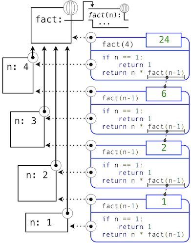
As the recursion "unwinds" through successive applications of the fact function to simpler and simpler problem instances, the result is eventually built starting from the base case. The diagram below shows how the recursion ends by passing the argument 1 to fact, and how the result of each call depends on the next until the base case is reached.

While we can unwind the recursion using our model of computation, it is often clearer to think about recursive calls as functional abstractions. That is, we should not care about how fact(n-1) is implemented in the body of fact; we should simply trust that it computes the factorial of n-1. Treating a recursive call as a functional abstraction has been called a recursive leap of faith. We define a function in terms of itself, but simply trust that the simpler cases will work correctly when verifying the correctness of the function. In this example, we trust that fact(n-1) will correctly compute (n-1)!; we must only check that n! is computed correctly if this assumption holds. In this way, verifying the correctness of a recursive function is a form of proof by induction.

The functions fact_iter and fact also differ because the former must introduce two additional names, total and k, that are not required in the recursive implementation. In general, iterative functions must maintain some local state that changes throughout the course of computation. At any point in the iteration, that state characterizes the result of completed work and the amount of work remaining. For example, when k is 3 and total is 2, there are still two terms remaining to be processed, 3 and 4. On the other hand, fact is characterized by its single argument n. The state of the computation is entirely contained within the structure of the expression tree, which has return values that take the role of total, and binds n to different values in different frames rather than explicitly tracking k.

Recursive functions can rely more heavily on the interpreter itself, by storing the state of the computation as part of the expression tree and environment, rather than explicitly using names in the local frame. For this reason, recursive functions are often easier to define, because we do not need to try to determine the local state that must be maintained across iterations. On the other hand, learning to recognize the computational processes evolved by recursive functions can require some practice.

3.2.3 Tree Recursion

Another common pattern of computation is called tree recursion. As an example, consider computing the sequence of Fibonacci numbers, in which each number is the sum of the preceding two.

>>> def fib(n):
        if n == 1:
            return 0
        if n == 2:
            return 1
        return fib(n-2) + fib(n-1)

>>> fib(6)
5

This recursive definition is tremendously appealing relative to our previous attempts: it exactly mirrors the familiar definition of Fibonacci numbers. Consider the pattern of computation that results from evaluating fib(6), shown below. To compute fib(6), we compute fib(5) and fib(4). To compute fib(5), we compute fib(4) and fib(3). In general, the evolved process looks like a tree (the diagram below is not a full expression tree, but instead a simplified depiction of the process; a full expression tree would have the same general structure). Each blue dot indicates a completed computation of a Fibonacci number in the traversal of this tree.

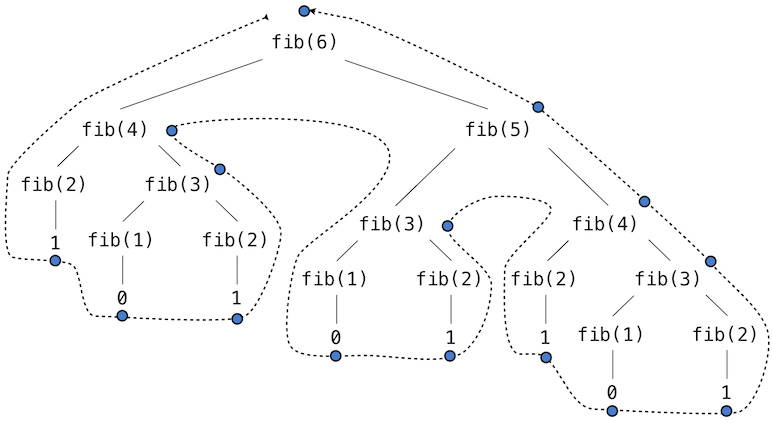
Functions that call themselves multiple times in this way are said to be tree recursive. This function is instructive as a prototypical tree recursion, but it is a terrible way to compute Fibonacci numbers because it does so much redundant computation. Notice that the entire computation of fib(4) -- almost half the work -- is duplicated. In fact, it is not hard to show that the number of times the function will compute fib(1) or fib(2) (the number of leaves in the tree, in general) is precisely fib(n+1). To get an idea of how bad this is, one can show that the value of fib(n) grows exponentially with n. Thus, the process uses a number of steps that grows exponentially with the input.

We have already seen an iterative implementation of Fibonacci numbers, repeated here for convenience.

>>> def fib_iter(n):
        prev, curr = 1, 0  # curr is the first Fibonacci number.
        for _ in range(n-1):
             prev, curr = curr, prev + curr
        return curr

The state that we must maintain in this case consists of the current and previous Fibonacci numbers. Implicitly the for statement also keeps track of the iteration count. This definition does not reflect the standard mathematical definition of Fibonacci numbers as clearly as the recursive approach. However, the amount of computation required in the iterative implementation is only linear in n, rather than exponential. Even for small values of n, this difference can be enormous.

One should not conclude from this difference that tree-recursive processes are useless. When we consider processes that operate on hierarchically structured data rather than numbers, we will find that tree recursion is a natural and powerful tool. Furthermore, tree-recursive processes can often be made more efficient.

Memoization. A powerful technique for increasing the efficiency of recursive functions that repeat computation is called memoization. A memoized function will store the return value for any arguments it has previously received. A second call to fib(4) would not evolve the same complex process as the first, but instead would immediately return the stored result computed by the first call.

Memoization can be expressed naturally as a higher-order function, which can also be used as a decorator. The definition below creates a cache of previously computed results, indexed by the arguments from which they were computed. The use of a dictionary will require that the argument to the memoized function be immutable in this implementation.

>>> def memo(f):
        """Return a memoized version of single-argument function f."""
        cache = {}
        def memoized(n):
            if n not in cache:
                cache[n] = f(n)
            return cache[n]
        return memoized

>>> fib = memo(fib)
>>> fib(40)
63245986

The amount of computation time saved by memoization in this case is substantial. The memoized, recursive fib function and the iterative fib_iter function both require an amount of time to compute that is only a linear function of their input n. To compute fib(40), the body of fib is executed 40 times, rather than 102,334,155 times in the unmemoized recursive case.

Space. To understand the space requirements of a function, we must specify generally how memory is used, preserved, and reclaimed in our environment model of computation. In evaluating an expression, we must preserve all active environments and all values and frames referenced by those environments. An environment is active if it provides the evaluation context for some expression in the current branch of the expression tree.

For example, when evaluating fib, the interpreter proceeds to compute each value in the order shown previously, traversing the structure of the tree. To do so, it only needs to keep track of those nodes that are above the current node in the tree at any point in the computation. The memory used to evaluate the rest of the branches can be reclaimed because it cannot affect future computation. In general, the space required for tree-recursive functions will be proportional to the maximum depth of the tree.

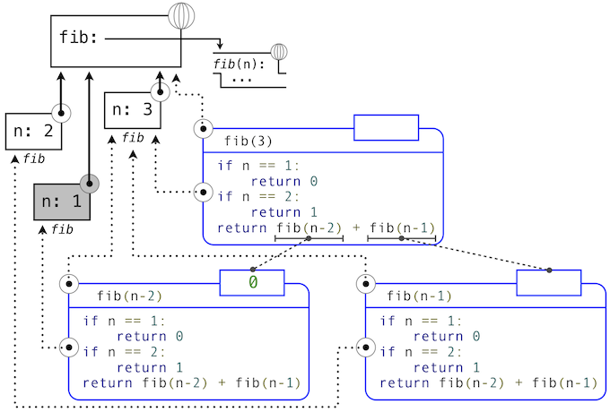
The diagram below depicts the environment and expression tree generated by evaluating fib(3). In the process of evaluating the return expression for the initial application of fib, the expression fib(n-2) is evaluated, yielding a value of 0. Once this value is computed, the corresponding environment frame (grayed out) is no longer needed: it is not part of an active environment. Thus, a well-designed interpreter can reclaim the memory that was used to store this frame. On the other hand, if the interpreter is currently evaluating fib(n-1), then the environment created by this application of fib (in which n is 2) is active. In turn, the environment originally created to apply fib to 3 is active because its value has not yet been successfully computed.

In the case of memo, the environment associated with the function it returns (which contains cache) must be preserved as long as some name is bound to that function in an active environment. The number of entries in the cache dictionary grows linearly with the number of unique arguments passed to fib, which scales linearly with the input. On the other hand, the iterative implementation requires only two numbers to be tracked during computation: prev and curr, giving it a constant size.

Memoization exemplifies a common pattern in programming that computation time can often be decreased at the expense of increased use of space, or vis versa.

3.2.4 Example: Counting Change

Consider the following problem: How many different ways can we make change of $1.00, given half-dollars, quarters, dimes, nickels, and pennies? More generally, can we write a function to compute the number of ways to change any given amount of money using any set of currency denominations?

This problem has a simple solution as a recursive function. Suppose we think of the types of coins available as arranged in some order, say from most to least valuable.

The number of ways to change an amount a using n kinds of coins equals

1. the number of ways to change a using all but the first kind of coin, plus
2. the number of ways to change the smaller amount a - d using all n kinds of coins, where d is the denomination of the first kind of coin.

To see why this is true, observe that the ways to make change can be divided into two groups: those that do not use any of the first kind of coin, and those that do. Therefore, the total number of ways to make change for some amount is equal to the number of ways to make change for the amount without using any of the first kind of coin, plus the number of ways to make change assuming that we do use the first kind of coin at least once. But the latter number is equal to the number of ways to make change for the amount that remains after using a coin of the first kind.

Thus, we can recursively reduce the problem of changing a given amount to the problem of changing smaller amounts using fewer kinds of coins. Consider this reduction rule carefully and convince yourself that we can use it to describe an algorithm if we specify the following base cases:

1. If a is exactly 0, we should count that as 1 way to make change.
2. If a is less than 0, we should count that as 0 ways to make change.
3. If n is 0, we should count that as 0 ways to make change.

We can easily translate this description into a recursive function:

>>> def count_change(a, kinds=(50, 25, 10, 5, 1)):
        """Return the number of ways to change amount a using coin kinds."""
        if a == 0:
            return 1
        if a < 0 or len(kinds) == 0:
            return 0
        d = kinds[0]
        return count_change(a, kinds[1:]) + count_change(a - d, kinds)

>>> count_change(100)
292

The count_change function generates a tree-recursive process with redundancies similar to those in our first implementation of fib. It will take quite a while for that 292 to be computed, unless we memoize the function. On the other hand, it is not obvious how to design an iterative algorithm for computing the result, and we leave this problem as a challenge.

3.2.5 Orders of Growth

The previous examples illustrate that processes can differ considerably in the rates at which they consume the computational resources of space and time. One convenient way to describe this difference is to use the notion of order of growth to obtain a coarse measure of the resources required by a process as the inputs become larger.

Let (n) be a parameter that measures the size of the problem, and let (R(n)) be the amount of resources the process requires for a problem of size (n). In our previous examples we took (n) to be the number for which a given function is to be computed, but there are other possibilities. For instance, if our goal is to compute an approximation to the square root of a number, we might take (n) to be the number of digits of accuracy required. In general there are a number of properties of the problem with respect to which it will be desirable to analyze a given process. Similarly, (R(n)) might measure the amount of memory used, the number of elementary machine operations performed, and so on. In computers that do only a fixed number of operations at a time, the time required to evaluate an expression will be proportional to the number of elementary machine operations performed in the process of evaluation.

We say that (R(n)) has order of growth (\Theta(f(n))), written (R(n) = \Theta(f(n))) (pronounced "theta of (f(n))"), if there are positive constants (k_1) and (k_2) independent of (n) such that

[k_1 \cdot f(n) \leq R(n) \leq k_2 \cdot f(n)]

for any sufficiently large value of (n). In other words, for large (n), the value (R(n)) is sandwiched between two values that both scale with (f(n)):

• A lower bound (k_1 \cdot f(n)) and
• An upper bound (k_2 \cdot f(n))

For instance, the number of steps to compute (n!) grows proportionally to the input (n). Thus, the steps required for this process grows as (\Theta(n)). We also saw that the space required for the recursive implementation fact grows as (\Theta(n)). By contrast, the iterative implementation fact_iter takes a similar number of steps, but the space it requires stays constant. In this case, we say that the space grows as (\Theta(1)).

The number of steps in our tree-recursive Fibonacci computation fib grows exponentially in its input (n). In particular, one can show that the nth Fibonacci number is the closest integer to

[\frac{\phi^{n-2}}{\sqrt{5}}]

where (\phi) is the golden ratio:

[\phi = \frac{1 + \sqrt{5}}{2} \approx 1.6180]

We also stated that the number of steps scales with the resulting value, and so the tree-recursive process requires (\Theta(\phi^n)) steps, a function that grows exponentially with (n).

Orders of growth provide only a crude description of the behavior of a process. For example, a process requiring (n^2) steps and a process requiring (1000 \cdot n^2) steps and a process requiring (3 \cdot n^2 + 10 \cdot n + 17) steps all have (\Theta(n^2)) order of growth. There are certainly cases in which an order of growth analysis is too coarse a method for deciding between two possible implementations of a function.

However, order of growth provides a useful indication of how we may expect the behavior of the process to change as we change the size of the problem. For a (\Theta(n)) (linear) process, doubling the size will roughly double the amount of resources used. For an exponential process, each increment in problem size will multiply the resource utilization by a constant factor. The next example examines an algorithm whose order of growth is logarithmic, so that doubling the problem size increases the resource requirement by only a constant amount.

3.2.6 Example: Exponentiation

Consider the problem of computing the exponential of a given number. We would like a function that takes as arguments a base b and a positive integer exponent n and computes (b^n). One way to do this is via the recursive definition

[\begin{array}{l l} b^n &= b \cdot b^{n-1} \ b^0 &= 1 \end{array}]

which translates readily into the recursive function

>>> def exp(b, n):
        if n == 0:
            return 1
        return b * exp(b, n-1)

This is a linear recursive process that requires (\Theta(n)) steps and (\Theta(n)) space. Just as with factorial, we can readily formulate an equivalent linear iteration that requires a similar number of steps but constant space.

>>> def exp_iter(b, n):
        result = 1
        for _ in range(n):
            result = result * b
        return result

We can compute exponentials in fewer steps by using successive squaring. For instance, rather than computing (b^8) as

[b \cdot (b \cdot (b \cdot (b \cdot (b \cdot (b \cdot (b \cdot b))))))]

we can compute it using three multiplications:

[\begin{array}{l l} b^2 &= b \cdot b \ b^4 &= b^2 \cdot b^2 \ b^8 &= b^4 \cdot b^4 \end{array}]

This method works fine for exponents that are powers of 2. We can also take advantage of successive squaring in computing exponentials in general if we use the recursive rule

[b^n = \left{\begin{array}{l l} (b^{\frac{1}{2} n})^2 & \mbox{if $n$ is even} \ b \cdot b^{n-1} & \mbox{if $n$ is odd} \end{array} \right.]

We can express this method as a recursive function as well:

>>> def square(x):
        return x*x

>>> def fast_exp(b, n):
        if n == 0:
            return 1
        if n % 2 == 0:
            return square(fast_exp(b, n//2))
        else:
            return b * fast_exp(b, n-1)

>>> fast_exp(2, 100)
1267650600228229401496703205376

The process evolved by fast_exp grows logarithmically with n in both space and number of steps. To see this, observe that computing (b^{2n}) using fast_exp requires only one more multiplication than computing (b^n). The size of the exponent we can compute therefore doubles (approximately) with every new multiplication we are allowed. Thus, the number of multiplications required for an exponent of n grows about as fast as the logarithm of n base 2. The process has (\Theta(\log n)) growth. The difference between (\Theta(\log n)) growth and (\Theta(n)) growth becomes striking as (n) becomes large. For example, fast_exp for n of 1000 requires only 14 multiplications instead of 1000.