1.6 Higher-Order Functions

We have seen that functions are, in effect, abstractions that describe compound operations independent of the particular values of their arguments. In square,

>>> def square(x):
        return x * x

we are not talking about the square of a particular number, but rather about a method for obtaining the square of any number. Of course we could get along without ever defining this function, by always writing expressions such as

>>> 3 * 3
9
>>> 5 * 5
25

and never mentioning square explicitly. This practice would suffice for simple computations like square, but would become arduous for more complex examples. In general, lacking function definition would put us at the disadvantage of forcing us to work always at the level of the particular operations that happen to be primitives in the language (multiplication, in this case) rather than in terms of higher-level operations. Our programs would be able to compute squares, but our language would lack the ability to express the concept of squaring. One of the things we should demand from a powerful programming language is the ability to build abstractions by assigning names to common patterns and then to work in terms of the abstractions directly. Functions provide this ability.

As we will see in the following examples, there are common programming patterns that recur in code, but are used with a number of different functions. These patterns can also be abstracted, by giving them names.

To express certain general patterns as named concepts, we will need to construct functions that can accept other functions as arguments or return functions as values. Functions that manipulate functions are called higher-order functions. This section shows how higher-order functions can serve as powerful abstraction mechanisms, vastly increasing the expressive power of our language.

1.6.1 Functions as Arguments

Consider the following three functions, which all compute summations. The first, sum_naturals, computes the sum of natural numbers up to n:

>>> def sum_naturals(n):
        total, k = 0, 1
        while k <= n:
            total, k = total + k, k + 1
        return total

>>> sum_naturals(100)
5050

The second, sum_cubes, computes the sum of the cubes of natural numbers up to n.

>>> def sum_cubes(n):
        total, k = 0, 1
        while k <= n:
            total, k = total + pow(k, 3), k + 1
        return total

>>> sum_cubes(100)
25502500

The third, pi_sum, computes the sum of terms in the series

which converges to pi very slowly.

>>> def pi_sum(n):
        total, k = 0, 1
        while k <= n:
            total, k = total + 8 / (k * (k + 2)), k + 4
        return total

>>> pi_sum(100)
3.121594652591009

These three functions clearly share a common underlying pattern. They are for the most part identical, differing only in name, the function of k used to compute the term to be added, and the function that provides the next value of k. We could generate each of the functions by filling in slots in the same template:

def <name>(n):
    total, k = 0, 1
    while k <= n:
        total, k = total + <term>(k), <next>(k)
    return total

The presence of such a common pattern is strong evidence that there is a useful abstraction waiting to be brought to the surface. Each of these functions is a summation of terms. As program designers, we would like our language to be powerful enough so that we can write a function that expresses the concept of summation itself rather than only functions that compute particular sums. We can do so readily in Python by taking the common template shown above and transforming the "slots" into formal parameters:

>>> def summation(n, term, next):
        total, k = 0, 1
        while k <= n:
            total, k = total + term(k), next(k)
        return total

Notice that summation takes as its arguments the upper bound n together with the functions term and next. We can use summation just as we would any function, and it expresses summations succinctly:

>>> def cube(k):
        return pow(k, 3)

>>> def successor(k):
        return k + 1

>>> def sum_cubes(n):
        return summation(n, cube, successor)

>>> sum_cubes(3)
36

Using an identity function that returns its argument, we can also sum integers.

>>> def identity(k):
        return k

>>> def sum_naturals(n):
        return summation(n, identity, successor)

>>> sum_naturals(10)
55

We can also define pi_sum piece by piece, using our summation abstraction to combine components.

>>> def pi_term(k):
        denominator = k * (k + 2)
        return 8 / denominator

>>> def pi_next(k):
        return k + 4

>>> def pi_sum(n):
        return summation(n, pi_term, pi_next)

>>> pi_sum(1e6)
3.1415906535898936

1.6.2 Functions as General Methods

We introduced user-defined functions as a mechanism for abstracting patterns of numerical operations so as to make them independent of the particular numbers involved. With higher-order functions, we begin to see a more powerful kind of abstraction: some functions express general methods of computation, independent of the particular functions they call.

Despite this conceptual extension of what a function means, our environment model of how to evaluate a call expression extends gracefully to the case of higher-order functions, without change. When a user-defined function is applied to some arguments, the formal parameters are bound to the values of those arguments (which may be functions) in a new local frame.

Consider the following example, which implements a general method for iterative improvement and uses it to compute the golden ratio. An iterative improvement algorithm begins with a guess of a solution to an equation. It repeatedly applies an update function to improve that guess, and applies a test to check whether the current guess is "close enough" to be considered correct.

>>> def iter_improve(update, test, guess=1):
        while not test(guess):
            guess = update(guess)
        return guess

The test function typically checks whether two functions, f and g, are near to each other for the value guess. Testing whether f(x) is near to g(x) is again a general method of computation.

>>> def near(x, f, g):
        return approx_eq(f(x), g(x))

A common way to test for approximate equality in programs is to compare the absolute value of the difference between numbers to a small tolerance value.

>>> def approx_eq(x, y, tolerance=1e-5):
        return abs(x - y) < tolerance

The golden ratio, often called phi, is a number that appears frequently in nature, art, and architecture. It can be computed via iter_improve using the golden_update, and it converges when its successor is equal to its square.

>>> def golden_update(guess):
        return 1/guess + 1

>>> def golden_test(guess):
        return near(guess, square, successor)

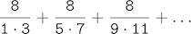
At this point, we have added several bindings to the global frame. The depictions of function values are abbreviated for clarity.

Calling iter_improve with the arguments golden_update and golden_test will compute an approximation to the golden ratio.

>>> iter_improve(golden_update, golden_test)
1.6180371352785146

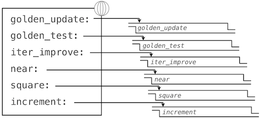
By tracing through the steps of our evaluation procedure, we can see how this result is computed. First, a local frame for iter_improve is constructed with bindings for update, test, and guess. In the body of iter_improve, the name test is bound to golden_test, which is called on the initial value of guess. In turn, golden_test calls near, creating a third local frame that binds the formal parameters f and g to square and successor.

Completing the evaluation of near, we see that the golden_test is False because 1 is not close to 2. Hence, evaluation proceeds with the suite of the while clause, and this mechanical process repeats several times.

This extended example illustrates two related big ideas in computer science. First, naming and functions allow us to abstract away a vast amount of complexity. While each function definition has been trivial, the computational process set in motion by our evaluation procedure appears quite intricate, and we didn't even illustrate the whole thing. Second, it is only by virtue of the fact that we have an extremely general evaluation procedure that small components can be composed into complex processes. Understanding that procedure allows us to validate and inspect the process we have created.

As always, our new general method iter_improve needs a test to check its correctness. The golden ratio can provide such a test, because it also has an exact closed-form solution, which we can compare to this iterative result.

>>> phi = 1/2 + pow(5, 1/2)/2
>>> def near_test():
        assert near(phi, square, successor), 'phi * phi is not near phi + 1'

>>> def iter_improve_test():
        approx_phi = iter_improve(golden_update, golden_test)
        assert approx_eq(phi, approx_phi), 'phi differs from its approximation'

New environment Feature: Higher-order functions.

Extra for experts. We left out a step in the justification of our test. For what range of tolerance values e can you prove that if near(x, square, successor) is true with tolerance value e, then approx_eq(phi, x) is true with the same tolerance?

1.6.3 Defining Functions III: Nested Definitions

The above examples demonstrate how the ability to pass functions as arguments significantly enhances the expressive power of our programming language. Each general concept or equation maps onto its own short function. One negative consequence of this approach to programming is that the global frame becomes cluttered with names of small functions. Another problem is that we are constrained by particular function signatures: the update argument to iter_improve must take exactly one argument. In Python, nested function definitions address both of these problems, but require us to amend our environment model slightly.

Let's consider a new problem: computing the square root of a number. Repeated application of the following update converges to the square root of x:

>>> def average(x, y):
        return (x + y)/2

>>> def sqrt_update(guess, x):
        return average(guess, x/guess)

This two-argument update function is incompatible with iter_improve, and it just provides an intermediate value; we really only care about taking square roots in the end. The solution to both of these issues is to place function definitions inside the body of other definitions.

>>> def square_root(x):
        def update(guess):
            return average(guess, x/guess)
        def test(guess):
            return approx_eq(square(guess), x)
        return iter_improve(update, test)

Like local assignment, local def statements only affect the current local frame. These functions are only in scope while square_root is being evaluated. Consistent with our evaluation procedure, these local def statements don't even get evaluated until square_root is called.

Lexical scope. Locally defined functions also have access to the name bindings in the scope in which they are defined. In this example, update refers to the name x, which is a formal parameter of its enclosing function square_root. This discipline of sharing names among nested definitions is called lexical scoping. Critically, the inner functions have access to the names in the environment where they are defined (not where they are called).

We require two extensions to our environment model to enable lexical scoping.

1. Each user-defined function has an associated environment: the environment in which it was defined.
2. When a user-defined function is called, its local frame extends the environment associated with the function.

Previous to square_root, all functions were defined in the global environment, and so they were all associated with the global environment. When we evaluate the first two clauses of square_root, we create functions that are associated with a local environment. In the call

>>> square_root(256)
16.00000000000039

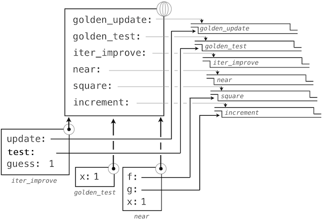
the environment first adds a local frame for square_root and evaluates the def statements for update and test (only update is shown).

Subsequently, the name update resolves to this newly defined function, which is passed as an argument to iter_improve. Within the body of iter_improve, we must apply our update function to the initial guess of 1. This final application creates an environment for update that begins with a local frame containing only g, but with the preceding frame for square_root still containing a binding for x.

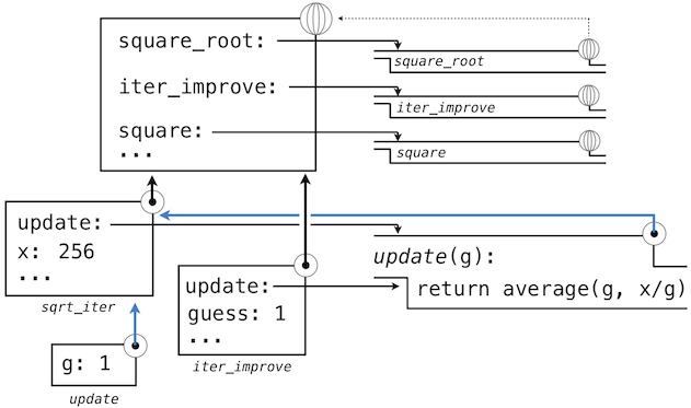
The most crucial part of this evaluation procedure is the transfer of an environment associated with a function to the local frame in which that function is evaluated. This transfer is highlighted by the blue arrows in this diagram.

In this way, the body of update can resolve a value for x. Hence, we realize two key advantages of lexical scoping in Python.

• The names of a local function do not interfere with names external to the function in which it is defined, because the local function name will be bound in the current local environment in which it is defined, rather than the global environment.
• A local function can access the environment of the enclosing function. This is because the body of the local function is evaluated in an environment that extends the evaluation environment in which it is defined.

The update function carries with it some data: the values referenced in the environment in which it was defined. Because they enclose information in this way, locally defined functions are often called closures.

New environment Feature: Local function definition.

1.6.4 Functions as Returned Values

We can achieve even more expressive power in our programs by creating functions whose returned values are themselves functions. An important feature of lexically scoped programming languages is that locally defined functions keep their associated environment when they are returned. The following example illustrates the utility of this feature.

With many simple functions defined, function composition is a natural method of combination to include in our programming language. That is, given two functions f(x) and g(x), we might want to define h(x) = f(g(x)). We can define function composition using our existing tools:

>>> def compose1(f, g):
        def h(x):
            return f(g(x))
        return h

>>> add_one_and_square = compose1(square, successor)
>>> add_one_and_square(12)
169

The 1 in compose1 indicates that the composed functions and returned result all take 1 argument. This naming convention isn't enforced by the interpreter; the 1 is just part of the function name.

At this point, we begin to observe the benefits of our investment in a rich model of computation. No modifications to our environment model are required to support our ability to return functions in this way.

1.6.5 Lambda Expressions

So far, every time we want to define a new function, we need to give it a name. But for other types of expressions, we don’t need to associate intermediate products with a name. That is, we can compute a*b + c*d without having to name the subexpressions a*b or c*d, or the full expression. In Python, we can create function values on the fly using lambda expressions, which evaluate to unnamed functions. A lambda expression evaluates to a function that has a single return expression as its body. Assignment and control statements are not allowed.

Lambda expressions are limited: They are only useful for simple, one-line functions that evaluate and return a single expression. In those special cases where they apply, lambda expressions can be quite expressive.

>>> def compose1(f,g):
        return lambda x: f(g(x))

We can understand the structure of a lambda expression by constructing a corresponding English sentence:

     lambda            x            :          f(g(x))
"A function that    takes x    and returns     f(g(x))"

Some programmers find that using unnamed functions from lambda expressions is shorter and more direct. However, compound lambda expressions are notoriously illegible, despite their brevity. The following definition is correct, but some programmers have trouble understanding it quickly.

>>> compose1 = lambda f,g: lambda x: f(g(x))

In general, Python style prefers explicit def statements to lambda expressions, but allows them in cases where a simple function is needed as an argument or return value.

Such stylistic rules are merely guidelines; you can program any way you wish. However, as you write programs, think about the audience of people who might read your program one day. If you can make your program easier to interpret, you will do those people a favor.

The term lambda is a historical accident resulting from the incompatibility of written mathematical notation and the constraints of early type-setting systems.

> It may seem perverse to use lambda to introduce a procedure/function. The notation goes back to Alonzo Church, who in the 1930's started with a "hat" symbol; he wrote the square function as "? . y × y". But frustrated typographers moved the hat to the left of the parameter and changed it to a capital lambda: "Λy . y × y"; from there the capital lambda was changed to lowercase, and now we see "λy . y × y" in math books and (lambda (y) (* y y)) in Lisp. > > —Peter Norvig (norvig.com/lispy2.html)

Despite their unusual etymology, lambda expressions and the corresponding formal language for function application, the lambda calculus, are fundamental computer science concepts shared far beyond the Python programming community. We will revisit this topic when we study the design of interpreters in Chapter 3.

1.6.6 Example: Newton's Method

This final extended example shows how function values, local defintions, and lambda expressions can work together to express general ideas concisely.

Newton's method is a classic iterative approach to finding the arguments of a mathematical function that yield a return value of 0. These values are called roots of a single-argument mathematical function. Finding a root of a function is often equivalent to solving a related math problem.

• The square root of 16 is the value x such that: square(x) - 16 = 0
• The log base 2 of 32 (i.e., the exponent to which we would raise 2 to get 32) is the value x such that: pow(2, x) - 32 = 0

Thus, a general method for finding roots will also provide us an algorithm to compute square roots and logarithms. Moreover, the equations for which we want to compute roots only contain simpler operations: multiplication and exponentiation.

A comment before we proceed: it is easy to take for granted the fact that we know how to compute square roots and logarithms. Not just Python, but your phone, your pocket calculator, and perhaps even your watch can do so for you. However, part of learning computer science is understanding how quantities like these can be computed, and the general approach presented here is applicable to solving a large class of equations beyond those built into Python.

Before even beginning to understand Newton's method, we can start programming; this is the power of functional abstractions. We simply translate our previous statements into code.

>>> def square_root(a):
        return find_root(lambda x: square(x) - a)

>>> def logarithm(a, base=2):
        return find_root(lambda x: pow(base, x) - a)

Of course, we cannot apply any of these functions until we define find_root, and so we need to understand how Newton's method works.

Newton's method is also an iterative improvement algorithm: it improves a guess of the root for any function that is differentiable. Notice that both of our functions of interest change smoothly; graphing x versus f(x) for

• f(x) = square(x) - 16 (light curve)
• f(x) = pow(2, x) - 32 (dark curve)

on a 2-dimensional plane shows that both functions produce a smooth curve without kinks that crosses 0 at the appropriate point.

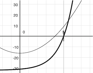
Because they are smooth (differentiable), these curves can be approximated by a line at any point. Newton's method follows these linear approximations to find function roots.

Imagine a line through the point (x, f(x)) that has the same slope as the curve for function f(x) at that point. Such a line is called the tangent, and its slope is called the derivative of f at x.

This line's slope is the ratio of the change in function value to the change in function argument. Hence, translating x by f(x) divided by the slope will give the argument value at which this tangent line touches 0.

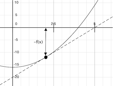
Our Newton update expresses the computational process of following this tangent line to 0. We approximate the derivative of the function by computing its slope over a very small interval.

>>> def approx_derivative(f, x, delta=1e-5):
        df = f(x + delta) - f(x)
        return df/delta

>>> def newton_update(f):
        def update(x):
            return x - f(x) / approx_derivative(f, x)
        return update

Finally, we can define the find_root function in terms of newton_update, our iterative improvement algorithm, and a test to see if f(x) is near 0. We supply a larger initial guess to improve performance for logarithm.

>>> def find_root(f, initial_guess=10):
        def test(x):
            return approx_eq(f(x), 0)
        return iter_improve(newton_update(f), test, initial_guess)

>>> square_root(16)
4.000000000026422
>>> logarithm(32, 2)
5.000000094858201

As you experiment with Newton's method, be aware that it will not always converge. The initial guess of iter_improve must be sufficiently close to the root, and various conditions about the function must be met. Despite this shortcoming, Newton's method is a powerful general computational method for solving differentiable equations. In fact, very fast algorithms for logarithms and large integer division employ variants of the technique.

1.6.7 Abstractions and First-Class Functions

We began this section with the observation that user-defined functions are a crucial abstraction mechanism, because they permit us to express general methods of computing as explicit elements in our programming language. Now we've seen how higher-order functions permit us to manipulate these general methods to create further abstractions.

As programmers, we should be alert to opportunities to identify the underlying abstractions in our programs, to build upon them, and generalize them to create more powerful abstractions. This is not to say that one should always write programs in the most abstract way possible; expert programmers know how to choose the level of abstraction appropriate to their task. But it is important to be able to think in terms of these abstractions, so that we can be ready to apply them in new contexts. The significance of higher-order functions is that they enable us to represent these abstractions explicitly as elements in our programming language, so that they can be handled just like other computational elements.

In general, programming languages impose restrictions on the ways in which computational elements can be manipulated. Elements with the fewest restrictions are said to have first-class status. Some of the "rights and privileges" of first-class elements are:

1. They may be bound to names.
2. They may be passed as arguments to functions.
3. They may be returned as the results of functions.
4. They may be included in data structures.

Python awards functions full first-class status, and the resulting gain in expressive power is enormous. Control structures, on the other hand, do not: you cannot pass if to a function the way you can sum.

1.6.8 Function Decorators

Python provides special syntax to apply higher-order functions as part of executing a def statement, called a decorator. Perhaps the most common example is a trace.

>>> def trace1(fn):
        def wrapped(x):
            print('-> ', fn, '(', x, ')')
            return fn(x)
        return wrapped

>>> @trace1
    def triple(x):
        return 3 * x

>>> triple(12)
->  <function triple at 0x102a39848> ( 12 )
36

In this example, A higher-order function trace1 is defined, which returns a function that precedes a call to its argument with a print statement that outputs the argument. The def statement for triple has an annototation, @trace1, which affects the execution rule for def. As usual, the function triple is created. However, the name triple is not bound to this function. Instead, the name triple is bound to the returned function value of calling trace1 on the newly defined triple function. In code, this decorator is equivalent to:

>>> def triple(x):
        return 3 * x

>>> triple = trace1(triple)

In the projects for this course, decorators are used for tracing, as well as selecting which functions to call when a program is run from the command line.

Extra for experts. The actual rule is that the decorator symbol @ may be followed by an expression (@trace1 is just a simple expression consisting of a single name). Any expression producing a suitable value is allowed. For example, with a suitable definition, you could define a decorator check_range so that decorating a function definition with @check_range(1, 10) would cause the function's results to be checked to make sure they are integers between 1 and 10. The call check_range(1,10) would return a function that would then be applied to the newly defined function before it is bound to the name in the def statement. A short tutorial on decorators by Ariel Ortiz gives further examples for interested students.