量化分析师的Python日记【第13天 Q Quant兵器谱之偏微分方程3】
来源:https://uqer.io/community/share/555dc9e8f9f06c6c7404f96e
欢迎来到 Black - Scholes — Merton 的世界!本篇中我们将使用在第11天学习到的知识应用到这个金融学的具体方程之上!
import numpy as np
import math
import seaborn as sns
from matplotlib import pylab
font.set_size(15)
1. 问题的提出
BSM模型可以设置为如下的偏微分方差初值问题:
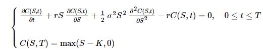
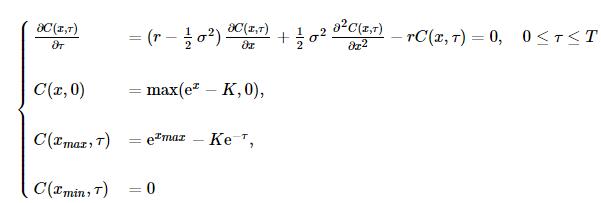
做变量替换τ=T−t,并且设置上下边界条件:
2. 算法
按照之前介绍的隐式差分格式的方法,用离散差分格式代替连续微分:
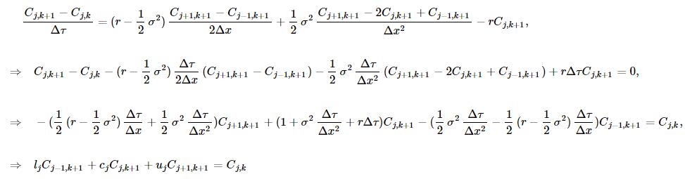
其中
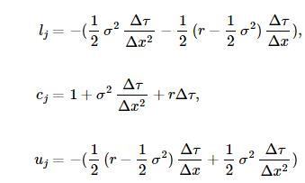
以上即为差分方程组。
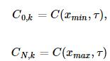
这里有些细节需要处理,就是左右边界条件,我们这里使用Dirichlet边界条件,则:
3.实现
import scipy as sp
from scipy.linalg import solve_banded
描述BSM方程结构的类:BSMModel
class BSMModel:

    def __init__(self, s0, r, sigma):
        self.s0 = s0
        self.x0 = math.log(s0)
        self.r = r
        self.sigma = sigma

    def log_expectation(self, T):
        return self.x0 + (self.r - 0.5 * self.sigma * self.sigma) * T

    def expectation(self, T):
        return math.exp(self.log_expectation(T))

    def x_max(self, T):
        return self.log_expectation(T) + 4.0 * self.sigma * math.sqrt(T)

    def x_min(self, T):
        return self.log_expectation(T) - 4.0 * self.sigma * math.sqrt(T)
描述我们这里设计到的产品的类:CallOption
class CallOption:

    def __init__(self, strike):
        self.k = strike

    def ic(self, spot):
        return max(spot - self.k, 0.0)

    def bcl(self, spot, tau, model):
        return 0.0

    def bcr(self, spot, tau, model):
        return spot - math.exp(-model.r*tau) * self.k
完整的隐式格式:BSMScheme
class BSMScheme:
    def __init__(self, model, payoff, T, M, N):
        self.model = model
        self.T = T
        self.M = M
        self.N = N
        self.dt = self.T / self.M
        self.payoff = payoff
        self.x_min = model.x_min(self.T)
        self.x_max = model.x_max(self.T)
        self.dx = (self.x_max - self.x_min) / self.N
        self.C = np.zeros((self.N+1, self.M+1)) # 全部网格
        self.xArray = np.linspace(self.x_min, self.x_max, self.N+1)
        self.C[:,0] = map(self.payoff.ic, np.exp(self.xArray))

        sigma_square = self.model.sigma*self.model.sigma
        r = self.model.r

        self.l_j = -(0.5*sigma_square*self.dt/self.dx/self.dx - 0.5 * (r - 0.5 * sigma_square)*self.dt/self.dx)
        self.c_j = 1.0 + sigma_square*self.dt/self.dx/self.dx + r*self.dt
        self.u_j = -(0.5*sigma_square*self.dt/self.dx/self.dx + 0.5 * (r - 0.5 * sigma_square)*self.dt/self.dx)

    def roll_back(self):

        for k in range(0, self.M):
            udiag = np.ones(self.N-1) * self.u_j
            ldiag =  np.ones(self.N-1) * self.l_j
            cdiag =  np.ones(self.N-1) * self.c_j

            mat = np.zeros((3,self.N-1))
            mat[0,:] = udiag
            mat[1,:] = cdiag
            mat[2,:] = ldiag
            rhs = np.copy(self.C[1:self.N,k])

            # 应用左端边值条件
            v1 = self.payoff.bcl(math.exp(self.x_min), (k+1)*self.dt, self.model)
            rhs[0] -= self.l_j * v1

            # 应用右端边值条件
            v2 = self.payoff.bcr(math.exp(self.x_max), (k+1)*self.dt, self.model)
            rhs[-1] -= self.u_j * v2

            x = solve_banded((1,1), mat, rhs)
            self.C[1:self.N, k+1] = x
            self.C[0][k+1] = v1
            self.C[self.N][k+1] = v2

    def mesh_grids(self):
        tArray = np.linspace(0, self.T, self.M+1)
        tGrids, xGrids = np.meshgrid(tArray, self.xArray)
        return tGrids, xGrids
应用在一起:
model = BSMModel(100.0, 0.05, 0.2)
payoff = CallOption(105.0)
scheme = BSMScheme(model, payoff, 5.0, 100, 300)
scheme.roll_back()
from matplotlib import pylab
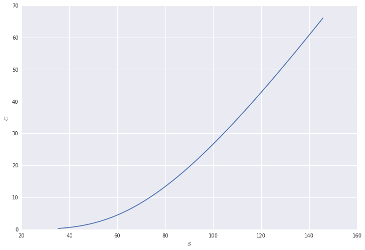
pylab.figure(figsize=(12,8))
pylab.plot(np.exp(scheme.xArray)[50:170], scheme.C[50:170,-1])
pylab.xlabel('$S$')
pylab.ylabel('$C$')
<matplotlib.text.Text at 0x76ea7d0>
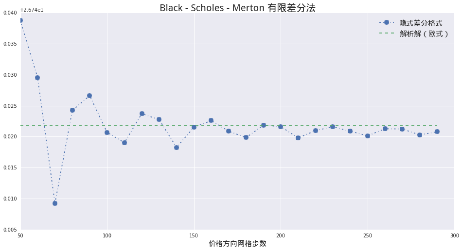
4. 收敛性测试
首先使用BSM模型的解析解获得精确解:
analyticPrice = BSMPrice(1, 105., 100., 0.05, 0.0, 0.2, 5.)
analyticPrice
| price | delta | gamma | vega | rho | theta | |
|---|---|---|---|---|---|---|
| 1 | 26.761844 | 0.749694 | 0.00711 | 71.10319 | 241.037549 | -3.832439 |
我们固定时间方向网格数为3000,分别计算不同S网格数情形下的结果:
xSteps = range(50,300,10)
finiteResult = []
for xStep in xSteps:
    model = BSMModel(100.0, 0.05, 0.2)
    payoff = CallOption(105.0)
    scheme = BSMScheme(model, payoff, 5.0, 3000, xStep)
    scheme.roll_back()

    interp = CubicNaturalSpline(np.exp(scheme.xArray), scheme.C[:,-1])
    price = interp(100.0)
    finiteResult.append(price)
我们可以画下收敛图:
anyRes = [analyticPrice['price'][1]] * len(xSteps)

pylab.figure(figsize = (16,8))
pylab.plot(xSteps, finiteResult, '-.', marker = 'o', markersize = 10)
pylab.plot(xSteps, anyRes, '--')
pylab.legend([u'隐式差分格式', u'解析解(欧式)'], prop = font)
pylab.xlabel(u'价格方向网格步数', fontproperties = font)
pylab.title(u'Black - Scholes - Merton 有限差分法', fontproperties = font, fontsize = 20)

<matplotlib.text.Text at 0x7857bd0>