Conservative Bollinger Bands
来源:https://uqer.io/community/share/548575def9f06c8e77336728
import quartz
import quartz.backtest    as qb
import quartz.performance as qp
from   quartz.api         import *

import pandas as pd
import numpy  as np
from datetime   import datetime
from matplotlib import pylab

import talib
start = datetime(2011, 1, 1)
end = datetime(2014, 8, 1)
benchmark = 'HS300'
universe = ['601398.XSHG', '600028.XSHG', '601988.XSHG', '600036.XSHG', '600030.XSHG',
            '601318.XSHG', '600000.XSHG', '600019.XSHG', '600519.XSHG', '601166.XSHG']
capital_base = 1000000
refresh_rate = 5
window = 200

def initialize(account):
    account.amount = 10000
    account.universe = universe
    add_history('hist', window)

def handle_data(account, data):

    for stk in account.universe:
        prices = account.hist[stk]['closePrice']
        if prices is None:
            return

        mu = prices.mean()
        sd = prices.std()

        upper = mu + 1*sd
        middle = mu
        lower = mu - 1*sd


        cur_pos = account.position.stkpos.get(stk, 0)
        cur_prc = prices[-1]
        if cur_prc > upper and cur_pos >= 0:
            order_to(stk, 0)
        if cur_prc < lower and cur_pos <= 0:
            order(stk, account.amount)
bt
|
tradeDate |
cash |
stock_position |
portfolio_value |
benchmark_return |
blotter |
| 0 |
2011-01-04 |
1000000 |
{} |
1000000 |
0.000000 |
[] |
| 1 |
2011-01-05 |
1000000 |
{} |
1000000 |
-0.004395 |
[] |
| 2 |
2011-01-06 |
1000000 |
{} |
1000000 |
-0.005044 |
[] |
| 3 |
2011-01-07 |
1000000 |
{} |
1000000 |
0.002209 |
[] |
| 4 |
2011-01-10 |
1000000 |
{} |
1000000 |
-0.018454 |
[] |
| 5 |
2011-01-11 |
1000000 |
{} |
1000000 |
0.005384 |
[] |
| 6 |
2011-01-12 |
1000000 |
{} |
1000000 |
0.005573 |
[] |
| 7 |
2011-01-13 |
1000000 |
{} |
1000000 |
-0.000335 |
[] |
| 8 |
2011-01-14 |
1000000 |
{} |
1000000 |
-0.015733 |
[] |
| 9 |
2011-01-17 |
1000000 |
{} |
1000000 |
-0.038007 |
[] |
| 10 |
2011-01-18 |
1000000 |
{} |
1000000 |
0.001109 |
[] |
| 11 |
2011-01-19 |
1000000 |
{} |
1000000 |
0.022569 |
[] |
| 12 |
2011-01-20 |
1000000 |
{} |
1000000 |
-0.032888 |
[] |
| 13 |
2011-01-21 |
1000000 |
{} |
1000000 |
0.013157 |
[] |
| 14 |
2011-01-24 |
1000000 |
{} |
1000000 |
-0.009795 |
[] |
| 15 |
2011-01-25 |
1000000 |
{} |
1000000 |
-0.005273 |
[] |
| 16 |
2011-01-26 |
1000000 |
{} |
1000000 |
0.013536 |
[] |
| 17 |
2011-01-27 |
1000000 |
{} |
1000000 |
0.016128 |
[] |
| 18 |
2011-01-28 |
1000000 |
{} |
1000000 |
0.003393 |
[] |
| 19 |
2011-01-31 |
1000000 |
{} |
1000000 |
0.013097 |
[] |
| 20 |
2011-02-01 |
1000000 |
{} |
1000000 |
0.000252 |
[] |
| 21 |
2011-02-09 |
1000000 |
{} |
1000000 |
-0.011807 |
[] |
| 22 |
2011-02-10 |
1000000 |
{} |
1000000 |
0.020788 |
[] |
| 23 |
2011-02-11 |
1000000 |
{} |
1000000 |
0.005410 |
[] |
| 24 |
2011-02-14 |
1000000 |
{} |
1000000 |
0.031461 |
[] |
| 25 |
2011-02-15 |
1000000 |
{} |
1000000 |
-0.000457 |
[] |
| 26 |
2011-02-16 |
1000000 |
{} |
1000000 |
0.009590 |
[] |
| 27 |
2011-02-17 |
1000000 |
{} |
1000000 |
-0.000807 |
[] |
| 28 |
2011-02-18 |
1000000 |
{} |
1000000 |
-0.010484 |
[] |
| 29 |
2011-02-21 |
1000000 |
{} |
1000000 |
0.014332 |
[] |
| 30 |
2011-02-22 |
1000000 |
{} |
1000000 |
-0.028954 |
[] |
| 31 |
2011-02-23 |
1000000 |
{} |
1000000 |
0.003529 |
[] |
| 32 |
2011-02-24 |
1000000 |
{} |
1000000 |
0.005101 |
[] |
| 33 |
2011-02-25 |
1000000 |
{} |
1000000 |
0.002094 |
[] |
| 34 |
2011-02-28 |
1000000 |
{} |
1000000 |
0.013117 |
[] |
| 35 |
2011-03-01 |
1000000 |
{} |
1000000 |
0.004733 |
[] |
| 36 |
2011-03-02 |
1000000 |
{} |
1000000 |
-0.003562 |
[] |
| 37 |
2011-03-03 |
1000000 |
{} |
1000000 |
-0.006654 |
[] |
| 38 |
2011-03-04 |
1000000 |
{} |
1000000 |
0.015193 |
[] |
| 39 |
2011-03-07 |
1000000 |
{} |
1000000 |
0.019520 |
[] |
| 40 |
2011-03-08 |
1000000 |
{} |
1000000 |
0.000884 |
[] |
| 41 |
2011-03-09 |
1000000 |
{} |
1000000 |
0.000420 |
[] |
| 42 |
2011-03-10 |
1000000 |
{} |
1000000 |
-0.017551 |
[] |
| 43 |
2011-03-11 |
1000000 |
{} |
1000000 |
-0.010025 |
[] |
| 44 |
2011-03-14 |
1000000 |
{} |
1000000 |
0.004787 |
[] |
| 45 |
2011-03-15 |
1000000 |
{} |
1000000 |
-0.018069 |
[] |
| 46 |
2011-03-16 |
1000000 |
{} |
1000000 |
0.013806 |
[] |
| 47 |
2011-03-17 |
1000000 |
{} |
1000000 |
-0.015730 |
[] |
| 48 |
2011-03-18 |
1000000 |
{} |
1000000 |
0.005813 |
[] |
| 49 |
2011-03-21 |
1000000 |
{} |
1000000 |
-0.002667 |
[] |
| 50 |
2011-03-22 |
1000000 |
{} |
1000000 |
0.004942 |
[] |
| 51 |
2011-03-23 |
1000000 |
{} |
1000000 |
0.013021 |
[] |
| 52 |
2011-03-24 |
1000000 |
{} |
1000000 |
-0.004155 |
[] |
| 53 |
2011-03-25 |
1000000 |
{} |
1000000 |
0.013263 |
[] |
| 54 |
2011-03-28 |
1000000 |
{} |
1000000 |
-0.001188 |
[] |
| 55 |
2011-03-29 |
1000000 |
{} |
1000000 |
-0.009905 |
[] |
| 56 |
2011-03-30 |
1000000 |
{} |
1000000 |
-0.000583 |
[] |
| 57 |
2011-03-31 |
1000000 |
{} |
1000000 |
-0.010071 |
[] |
| 58 |
2011-04-01 |
1000000 |
{} |
1000000 |
0.015339 |
[] |
| 59 |
2011-04-06 |
1000000 |
{} |
1000000 |
0.011714 |
[] |
| ... |
... |
... |
... |
... |
... |
868 rows × 6 columns
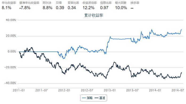
perf = qp.perf_parse(bt)
out_keys = ['annualized_return', 'volatility', 'information',
            'sharpe', 'max_drawdown', 'alpha', 'beta']

for k in out_keys:
    print '%s: %s' % (k, perf[k])

annualized_return: 0.0806072460858
volatility: 0.121542243584
information: 0.967129870018
sharpe: 0.344919139631
max_drawdown: 0.100359317734
alpha: 0.0876204656402
beta: 0.392712356147
perf['cumulative_return'].plot()
perf['benchmark_cumulative_return'].plot()
pylab.legend(['current_strategy','HS300'])
