10.3 Arch/Garch 模型 · 如何使用优矿进行 GARCH 模型分析
ARCH 建模示例
小弟近来学习波动率建模相关知识,正巧发现优矿中有ARCH包,所以通过翻译ARCH包文档中的示例,来学习相关函数用法。
翻译有不少不准确的地方,请大家指出,我会及时改进。
import numpy as np
import matplotlib.mlab as mlab
import matplotlib.pyplot as plt

try:
   import seaborn
except ImportError:
    pass
一、准备工作
这个例子中使用通联DataAPI提供的行情数据。以平安银行为例。
下面画出了平安银行从1990年到2015年收益率情况。
import datetime as dt
st = dt.datetime(1990,1,1)
en = dt.datetime(2015,6,30)

data = DataAPI.MktEqudGet(secID=u"",ticker=u"000001",tradeDate=u"",beginDate=u"",endDate=u"",field=u"ticker,secShortName,tradeDate,closePrice,PE",pandas="1")

# data.index = data.tradeDate
returns = 100 * data['closePrice'].pct_change().dropna()
figure = returns.plot(figsize=(20,6))

二、实现常见模型
描述一个模型最简单的方法就是使用Python的类库arch.arch_model。使用这个类库可以实现大多数常见的模型。
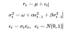
简单的调用arch类库会得到一个均值恒定,误差符合正态分布,符合GARCH(1,1)波动率过程的模型。
通过调用fit方法,可以对这个模型进行估计。可选输入项 update_freq控制优化器输出结果的频率,disp控制是否返回收敛相关信息。返回结果直接提供了估计的参数值和相关数量,同时包含估计结果的摘要信息。
GARCH (均值恒定)
使用默认选项,可以生成一个均值恒定,误差符合正态分布,同时符合GARCH(1,1)条件方差的模型。
通过拟合获得模型的参数,下面展示拟合结果的摘要。
from arch import arch_model
am = arch_model(returns)
res = am.fit(update_freq=5)
print(res.summary())

Iteration:      5,   Func. Count:     38,   Neg. LLF: 5787.7752693
Iteration:     10,   Func. Count:     75,   Neg. LLF: 5785.39088499
Optimization terminated successfully.    (Exit mode 0)
            Current function value: 5785.0196556
            Iterations: 14
            Function evaluations: 101
            Gradient evaluations: 14
                     Constant Mean - GARCH Model Results
==============================================================================
Dep. Variable:             closePrice   R-squared:                      -0.000
Mean Model:             Constant Mean   Adj. R-squared:                 -0.000
Vol Model:                      GARCH   Log-Likelihood:               -5785.02
Distribution:                  Normal   AIC:                           11578.0
Method:            Maximum Likelihood   BIC:                           11601.1
                                        No. Observations:                 2373
Date:                Fri, Oct 16 2015   Df Residuals:                     2369
Time:                        11:08:36   Df Model:                            4
                                  Mean Model
==============================================================================
                 coef    std err          t      P>|t|        95.0% Conf. Int.
------------------------------------------------------------------------------
mu             0.0349  2.825e-03     12.348  4.985e-35   [2.935e-02,4.042e-02]
                               Volatility Model
==============================================================================
                 coef    std err          t      P>|t|        95.0% Conf. Int.
------------------------------------------------------------------------------
omega          0.0383  2.763e-03     13.861  1.085e-43   [3.288e-02,4.371e-02]
alpha[1]       0.0287  2.439e-04    117.761      0.000   [2.825e-02,2.920e-02]
beta[1]        0.9694  4.516e-04   2146.801      0.000       [  0.969,  0.970]
==============================================================================

Covariance estimator: robust
plot() 函数可以快速展示 标的的标准偏差和条件波动率。
fig = res.plot(annualize='D')

GJR-GARCH
arch_model 在构建模型时,还可以添加附加参数。在这个例子中,设置o为1, 即包含了非对称冲击的一阶滞后项,从而将原GARCH模型转换为一个GJR-GARCH模型。新的模型具有动态方差,由下面公式给出:
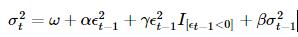
其中,I是一个指标函数,当它的输入参数为真时,返回为1.
对数似然函数值改进了非对称项引入的平稳性问题,从而使参数估计具有很高的显著性。
am = arch_model(returns, p=1, o=1, q=1)
res = am.fit(update_freq=5, disp='off')
print(res.summary())
TARCH/ZARCH
TARCH模型 (又称为 ZARCH模型) 是对波动率的绝对值进行建模. 使用该模型时,需要在arch_model建构函数中,设置power=1.0。因为默认的阶数为2,对应的是用平方项表示的方差变化过程。
TARCH model的波动率过程由下面公式给出:

更一般的情况,模型的动态波动率代码κ阶。这种情况由下面的公式给出
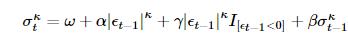
其中,条件方差为
尽管对数似然函数值变动范围更小,TARCH 模型还是对拟合过程做了改进。
am = arch_model(returns, p=1, o=1, q=1, power=1.0)
res = am.fit(update_freq=5)
print(res.summary())

Iteration:      5,   Func. Count:     45,   Neg. LLF: 5765.36462439
Iteration:     10,   Func. Count:     84,   Neg. LLF: 5758.70411096
Iteration:     15,   Func. Count:    121,   Neg. LLF: 5758.63601597
Optimization terminated successfully.    (Exit mode 0)
            Current function value: 5758.6360268
            Iterations: 15
            Function evaluations: 121
            Gradient evaluations: 15
                  Constant Mean - TARCH/ZARCH Model Results
==============================================================================
Dep. Variable:             closePrice   R-squared:                      -0.000
Mean Model:             Constant Mean   Adj. R-squared:                 -0.000
Vol Model:                TARCH/ZARCH   Log-Likelihood:               -5758.64
Distribution:                  Normal   AIC:                           11527.3
Method:            Maximum Likelihood   BIC:                           11556.1
                                        No. Observations:                 2373
Date:                Fri, Oct 16 2015   Df Residuals:                     2368
Time:                        12:50:24   Df Model:                            5
                                  Mean Model
==============================================================================
                 coef    std err          t      P>|t|        95.0% Conf. Int.
------------------------------------------------------------------------------
mu             0.0625  4.323e-03     14.456  2.296e-47   [5.402e-02,7.096e-02]
                               Volatility Model
==============================================================================
                 coef    std err          t      P>|t|        95.0% Conf. Int.
------------------------------------------------------------------------------
omega          0.0457  4.933e-03      9.257  2.107e-20   [3.599e-02,5.533e-02]
alpha[1]       0.0594  1.012e-03     58.701      0.000   [5.742e-02,6.139e-02]
gamma[1]      -0.0184  5.771e-04    -31.882 4.768e-223 [-1.953e-02,-1.727e-02]
beta[1]        0.9498  2.510e-03    378.466      0.000       [  0.945,  0.955]
==============================================================================

Covariance estimator: robust
学生T分布误差
金融资产回报率的分布往往体现出肥尾现象,学生T分布是一种简单的方法,可以用来捕捉这种特性。在调用arch_model 构建函数时,可以将概率分布从正态分布转换为学生T分布。
标准化的新息展示出,分布函数具有一个将近10个估计自由度的肥尾。 对数似然函数值同样有大的改善。
am = arch_model(returns, p=1, o=1, q=1, power=1.0, dist='StudentsT')
res = am.fit(update_freq=5)
print(res.summary())

Iteration:      5,   Func. Count:     48,   Neg. LLF: 5522.16193119
Iteration:     10,   Func. Count:     93,   Neg. LLF: 5475.09377571
Iteration:     15,   Func. Count:    138,   Neg. LLF: 5451.04968458
Iteration:     20,   Func. Count:    179,   Neg. LLF: 5435.39156625
Iteration:     25,   Func. Count:    223,   Neg. LLF: 5434.83467797
Iteration:     30,   Func. Count:    269,   Neg. LLF: 5434.83086355
Optimization terminated successfully.    (Exit mode 0)
            Current function value: 5434.83085822
            Iterations: 33
            Function evaluations: 304
            Gradient evaluations: 33
                     Constant Mean - TARCH/ZARCH Model Results
====================================================================================
Dep. Variable:                   closePrice   R-squared:                      -0.001
Mean Model:                   Constant Mean   Adj. R-squared:                 -0.001
Vol Model:                      TARCH/ZARCH   Log-Likelihood:               -5434.83
Distribution:      Standardized Student's t   AIC:                           10881.7
Method:                  Maximum Likelihood   BIC:                           10916.3
                                              No. Observations:                 2373
Date:                      Fri, Oct 16 2015   Df Residuals:                     2367
Time:                              13:04:54   Df Model:                            6
                                   Mean Model
===============================================================================
                  coef    std err          t      P>|t|        95.0% Conf. Int.
-------------------------------------------------------------------------------
mu         -1.3518e-08  1.493e-10    -90.539      0.000 [-1.381e-08,-1.323e-08]
                                Volatility Model
===============================================================================
                  coef    std err          t      P>|t|        95.0% Conf. Int.
-------------------------------------------------------------------------------
omega           0.0894      0.304      0.294      0.769       [ -0.507,  0.686]
alpha[1]        0.1185  9.143e-03     12.962  2.004e-38       [  0.101,  0.136]
gamma[1]   -2.9293e-03  4.117e-03     -0.712      0.477  [-1.100e-02,5.139e-03]
beta[1]         0.8829  9.652e-02      9.148  5.803e-20       [  0.694,  1.072]
                                 Distribution
==============================================================================
                 coef    std err          t      P>|t|        95.0% Conf. Int.
------------------------------------------------------------------------------
nu             3.6773      0.142     25.919 4.047e-148       [  3.399,  3.955]
==============================================================================

Covariance estimator: robust
使用固定参数
在一些场景下,相比估计出来的参数,使用固定参数可能更让人感兴趣。
使用arch_model的fix()可以同样生成一个模型。除了没有与推断相关的值(标准差,t统计量等)的差别之外,新的模型和通常的模型没有什么差别。
在这个例子中,将参数固定设置为之前估计模型的对称版本。
fixed_res = am.fix([0.0235, 0.01, 0.06, 0.0, 0.9382, 8.0])
print(fixed_res.summary())

                      Constant Mean - TARCH/ZARCH Model Results
=====================================================================================
Dep. Variable:                    closePrice   R-squared:                          --
Mean Model:                    Constant Mean   Adj. R-squared:                     --
Vol Model:                       TARCH/ZARCH   Log-Likelihood:               -5579.95
Distribution:       Standardized Student's t   AIC:                           11171.9
Method:            User-specified Parameters   BIC:                           11206.5
                                               No. Observations:                 2373
Date:                       Fri, Oct 16 2015
Time:                               13:04:57
      Mean Model
=====================
                 coef
---------------------
mu             0.0235
   Volatility Model
=====================
                 coef
---------------------
omega          0.0100
alpha[1]       0.0600
gamma[1]       0.0000
beta[1]        0.9382
     Distribution
=====================
                 coef
---------------------
nu             8.0000
=====================

Results generated with user-specified parameters.
Since the model was not estimated, there are no std. errors.
import pandas as pd
df = pd.concat([res.conditional_volatility,fixed_res.conditional_volatility],1)
df.columns = ['Estimated', 'Fixed']
df.plot()

<matplotlib.axes.AxesSubplot at 0x6b5cd90>

三、通过多个组件模块创建模型
模型同样可以使用代表三类模型的arch模块进行系统性的构建。
- A mean model (arch.mean)
- Zero mean (ZeroMean) - useful if using residuals from a model estimated separately
- Constant mean (ConstantMean) - common for most liquid financial assets
- Autoregressive (ARX) with optional exogenous regressors
- Heterogeneous (HARX) autoregression with optional exogenous regressors
- Exogenous regressors only (LS)
- A volatility process (arch.volatility)
- ARCH (ARCH)
- GARCH (GARCH)
- GJR-GARCH (GARCH using o argument)
- TARCH/ZARCH (GARCH using power argument set to 1)
- Power GARCH and Asymmetric Power GARCH (GARCH using power)
- Heterogeneous ARCH (HARCH)
- Parameterless Models
- Exponentially Weighted Moving Average Variance, known as RiskMetrics (EWMAVariance)
- Weighted averages of EWMAs, known as the RiskMetrics 2006 methodology (RiskMetrics2006)
- A distribution (arch.distribution)
- Normal (Normal)
- Standardized Students's T (StudentsT)
Mean Models 均值模型
第一种选择是使用均值模型。 对于很多流动性充足的金融资产来说, 恒定均值(甚至是0均值)的模型就足够了。
对于其他一些时间序列,若通货膨胀率数据,可能需要更加复杂的模型。 下面的例子使用了中国居民消费价格指数(CPI)数据。这些数据由通联DataAPI提供。
core_cpi = DataAPI.ChinaDataCPIGet(indicID=u"M030000003",indicName=u"",beginDate=u"20050101",endDate=u"",field=u"",pandas="1")
ann_inflation = 100 * core_cpi.sort(columns='periodDate').dataValue.pct_change(12).dropna()
fig = ann_inflation.plot()
fig

<matplotlib.axes.AxesSubplot at 0x6e6a090>

所有的均值模型都派生自恒定方差、正态分布误差的基础模型。
对于ARX模型,lags输入参数制定了模型需要包括的滞后项阶数。
from arch.univariate import ARX
ar = ARX(ann_inflation, lags = [1, 3, 12])
print(ar.fit().summary())

                     AR - Constant Variance Model Results
==============================================================================
Dep. Variable:              dataValue   R-squared:                       0.264
Mean Model:                        AR   Adj. R-squared:                  0.242
Vol Model:          Constant Variance   Log-Likelihood:               -685.867
Distribution:                  Normal   AIC:                           1381.73
Method:            Maximum Likelihood   BIC:                           1395.00
                                        No. Observations:                  105
Date:                Fri, Oct 16 2015   Df Residuals:                      100
Time:                        13:21:29   Df Model:                            5
                                    Mean Model
=================================================================================
                    coef    std err          t      P>|t|        95.0% Conf. Int.
---------------------------------------------------------------------------------
Const            -1.4076    254.081 -5.540e-03      0.996  [-4.994e+02,4.966e+02]
dataValue[1]      0.4233      0.112      3.777  1.590e-04       [  0.204,  0.643]
dataValue[3]      0.1590  1.423e-02     11.173  5.523e-29       [  0.131,  0.187]
dataValue[12]    -0.0117  1.050e-03    -11.133  8.695e-29 [-1.374e-02,-9.628e-03]
                               Volatility Model
==============================================================================
                 coef    std err          t      P>|t|        95.0% Conf. Int.
------------------------------------------------------------------------------
sigma2     2.7619e+04  2.259e+08  1.223e-04      1.000  [-4.427e+08,4.427e+08]
==============================================================================

Covariance estimator: White's Heteroskedasticity Consistent Estimator
Volatility Processes 波动率过程
波动率过程可以通过在均值模型中添加volatility属性来实现。
下面的例子中将模型的波动率设置为ARCH(5),update_freq和disp用来约束fit()进行估计时候的输出内容。
from arch.univariate import ARCH, GARCH
ar.volatility = ARCH(p=5)
res = ar.fit(update_freq=0, disp='off')
print(res.summary())

                           AR - ARCH Model Results
==============================================================================
Dep. Variable:              dataValue   R-squared:                       0.104
Mean Model:                        AR   Adj. R-squared:                  0.077
Vol Model:                       ARCH   Log-Likelihood:               -576.003
Distribution:                  Normal   AIC:                           1172.01
Method:            Maximum Likelihood   BIC:                           1198.55
                                        No. Observations:                  105
Date:                Fri, Oct 16 2015   Df Residuals:                       95
Time:                        13:25:52   Df Model:                           10
                                    Mean Model
=================================================================================
                    coef    std err          t      P>|t|        95.0% Conf. Int.
---------------------------------------------------------------------------------
Const           -11.9096     29.775     -0.400      0.689       [-70.268, 46.449]
dataValue[1]      0.8647  2.093e-02     41.313      0.000       [  0.824,  0.906]
dataValue[3]     -0.0296  9.925e-03     -2.978  2.904e-03 [-4.901e-02,-1.010e-02]
dataValue[12]    -0.0154  2.936e-04    -52.419      0.000 [-1.597e-02,-1.482e-02]
                                Volatility Model
===============================================================================
                  coef    std err          t      P>|t|        95.0% Conf. Int.
-------------------------------------------------------------------------------
omega         404.9890  1.164e+05  3.480e-03      0.997  [-2.277e+05,2.285e+05]
alpha[1]        0.6348  5.176e-02     12.266  1.383e-34       [  0.533,  0.736]
alpha[2]        0.2690  1.767e-02     15.221  2.552e-52       [  0.234,  0.304]
alpha[3]        0.0962  1.161e-02      8.283  1.196e-16     [7.341e-02,  0.119]
alpha[4]    2.5205e-10  3.554e-04  7.093e-07      1.000  [-6.965e-04,6.965e-04]
alpha[5]   -4.6303e-10  1.178e-05 -3.929e-05      1.000  [-2.310e-05,2.309e-05]
===============================================================================

Covariance estimator: robust
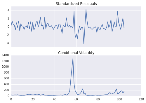
下面的图标,展示了标准化后的新息和条件波动率的情况。可以看出,虽然进行了标准化处理,一些位置还是出现了较大的误差(通过振幅来看)
fig = res.plot()
Distributions 概率分布情况
最后提一下,模型的概率分布可以通过设置distribution属性来修改,将默认的正态分布修改为学生T分布。
学生T分布改进了模型,模型的估计自由度大约在8左右。
备注 1 本文章是将Python ARCH类库的帮助文档进行翻译产生的。
本文将原文中的数据源替换为优矿/通联DataAPI的数据,方便优矿用户进行参照和分析。
2 文中,多次提到iter,但这个疑为原作者笔误,故都改为update_freq
3 原文最后一章‘WTI Crude’由于给出的例子和当前的arch包版本不兼容,无法正确运行,故没有引入