Vanishing & Exploding Gradients

gradients get smaller as algorithm progresses to lower layers. Eventually GD leaves lower weights virtually unchanged. so training never converges.
gradients can also grow out of control (often seen in RNNs).
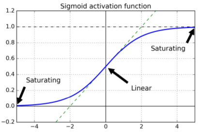
Significant paper - using combo of logistic sigmoid activiation with random weight initialization (normal, mean=0, stdev=1) -- output variance was >> input variance.
logistic activation: function saturates at 0 or 1 with derivative very close to 0 ==> so backpropagation has no gradient to use.

Xavier & He Initialization

For signals to flow properly in both directions, each layer's output variance should equal its input variance.
Recommends initializing connection weights with random settings using #ins, #outs
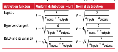
Default: fully_connected() function uses Xavier initialization w/ uniform distribution. Change to He initialization by using variance_scaling_initializer() function

import tensorflow as tf
from tensorflow.contrib.layers import fully_connected

n_inputs = 28*28
n_hidden1 = 300

X = tf.placeholder(tf.float32, shape=(None, n_inputs), name="X")

he_init = tf.contrib.layers.variance_scaling_initializer()
hidden1 = fully_connected(X, n_hidden1, weights_initializer=he_init, scope="h1")

Non-Saturating Activation Functions

ReLU activations suffer from dying ReLU problem (they stop emitting anything other than zero).
Workaround: the leaku ReLU. Alpha defines leakage; typical set to 0.01.
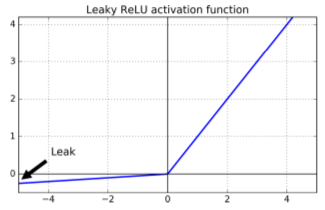
Also: randomized leaky ReLU (RReLU) (randomized alpha)
Also: parametric leaky RuLE (PReLU) (alpha can be modified during backprop)
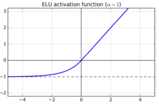
Also: exponential linear unit (ELU). Allows negative values when z<0; non-zero gradient for z<0 (avoids dying units issue); smooth function everywhere. Uses exponential function, so harder to compute. paper

# TF doesn't have leaky ReLU predefined, but easy to build.

def leaky_relu(z, name=None):
    return tf.maximum(0.01 * z, z, name=name)

hidden1 = fully_connected(X, n_hidden1, activation_fn=leaky_relu)

Batch Normalization

proposed to solve vanishing/exploding gradients.
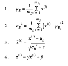
Idea: pror to activation function, 1) zero-center & normalize inputs 2) scale & shift result with 2 new params per layer
Net effect: model learns optimal scale & mean of inputs for each layer
Algorithm:
Does add computational complexity. Consider plain ELU + He initializaton as well.

Batch Normalization with TF

batch_normalization() - centers & normalizes inputs
batch_norm() - above, plus finds mean, stdev, scaling, offset params
call directly or include it in fully_connected() arguments

# use MNIST dataset again
from tensorflow.examples.tutorials.mnist import input_data
mnist = input_data.read_data_sets("/tmp/data/")

Successfully downloaded train-images-idx3-ubyte.gz 9912422 bytes.
Extracting /tmp/data/train-images-idx3-ubyte.gz
Successfully downloaded train-labels-idx1-ubyte.gz 28881 bytes.
Extracting /tmp/data/train-labels-idx1-ubyte.gz
Successfully downloaded t10k-images-idx3-ubyte.gz 1648877 bytes.
Extracting /tmp/data/t10k-images-idx3-ubyte.gz
Successfully downloaded t10k-labels-idx1-ubyte.gz 4542 bytes.
Extracting /tmp/data/t10k-labels-idx1-ubyte.gz

#setup

import tensorflow as tf
from tensorflow.contrib.layers import batch_norm, fully_connected

tf.reset_default_graph() 

n_inputs = 28 * 28
n_hidden1 = 300
n_hidden2 = 100
n_outputs = 10
learning_rate = 0.01

X = tf.placeholder(tf.float32, shape=(None, n_inputs), name="X")
y = tf.placeholder(tf.int64, shape=(None), name="y")

def leaky_relu(z, name=None):
  return tf.maximum(0.01 * z, z, name=name)

# is_training: tells batch_norm() whether to use current minibatch's mean & stdev 
# (found during training) or use running avgs (during testing)

with tf.name_scope("dnn"):
    hidden1 = fully_connected(X, n_hidden1, activation_fn=leaky_relu, scope="hidden1")
    hidden2 = fully_connected(hidden1, n_hidden2, activation_fn=leaky_relu, scope="hidden2")
    logits = fully_connected(hidden2, n_outputs, activation_fn=None, scope="outputs")

with tf.name_scope("loss"):
    xentropy = tf.nn.sparse_softmax_cross_entropy_with_logits(labels=y, logits=logits)
    loss = tf.reduce_mean(xentropy, name="loss")

with tf.name_scope("train"):
    optimizer = tf.train.GradientDescentOptimizer(learning_rate)
    training_op = optimizer.minimize(loss)

with tf.name_scope("eval"):
    correct = tf.nn.in_top_k(logits, y, 1)
    accuracy = tf.reduce_mean(tf.cast(correct, tf.float32))

init = tf.global_variables_initializer()
saver = tf.train.Saver()

n_epochs = 20
batch_size = 100

with tf.Session() as sess:

    init.run()

    for epoch in range(n_epochs):

        for iteration in range(len(mnist.test.labels)//batch_size):

            X_batch, y_batch = mnist.train.next_batch(batch_size)
            sess.run(training_op, feed_dict={X: X_batch, y: y_batch})

        acc_train = accuracy.eval(feed_dict={X: X_batch, y: y_batch})
        acc_test = accuracy.eval(feed_dict={X: mnist.test.images, y: mnist.test.labels})

        print(epoch, "Train accuracy:", acc_train, "Test accuracy:", acc_test)

    save_path = saver.save(sess, "my_model_final.ckpt")

0 Train accuracy: 0.6 Test accuracy: 0.642
1 Train accuracy: 0.73 Test accuracy: 0.7824
2 Train accuracy: 0.81 Test accuracy: 0.827
3 Train accuracy: 0.84 Test accuracy: 0.8539
4 Train accuracy: 0.8 Test accuracy: 0.8686
5 Train accuracy: 0.87 Test accuracy: 0.8759
6 Train accuracy: 0.85 Test accuracy: 0.8843
7 Train accuracy: 0.91 Test accuracy: 0.8903
8 Train accuracy: 0.86 Test accuracy: 0.8969
9 Train accuracy: 0.91 Test accuracy: 0.9018
10 Train accuracy: 0.91 Test accuracy: 0.9014
11 Train accuracy: 0.86 Test accuracy: 0.9065
12 Train accuracy: 0.88 Test accuracy: 0.9078
13 Train accuracy: 0.87 Test accuracy: 0.91
14 Train accuracy: 0.93 Test accuracy: 0.911
15 Train accuracy: 0.9 Test accuracy: 0.9123
16 Train accuracy: 0.91 Test accuracy: 0.9141
17 Train accuracy: 0.9 Test accuracy: 0.9149
18 Train accuracy: 0.92 Test accuracy: 0.9159
19 Train accuracy: 0.93 Test accuracy: 0.9174

Gradient Clipping

to limit exploding gradients problem. Clip during backprop.
Typical use case: recurrent NNs.
source
Uses TF minimize() function in optimizer.

threshold = 1.0

optimizer = tf.train.GradientDescentOptimizer(
    learning_rate)

grads_and_vars = optimizer.compute_gradients(
    loss)

capped_gvs = [
    (tf.clip_by_value(
        grad, -threshold, threshold), var)
    for grad, var in grads_and_vars]

training_op = optimizer.apply_gradients(capped_gvs)

Pretrained Layers & Reuse

best practice: look for existing NN that tackles similar task, then reuse lower layers (aka transfer learning).

# Reuse with TF

Reusing Models from Other Frameworks

Requires manual loading of weights (ex: Theano)
Very tedious

'''
original_w = [] # Load the weights from the other framework
original_b = [] # Load the biases from the other framework

X = tf.placeholder(tf.float32, shape=(None, n_inputs), name="X")
hidden1 = fully_connected(X, n_hidden1, scope="hidden1")

[...] # # Build the rest of the model

# Get a handle on the variables created by fully_connected()

with tf.variable_scope("", default_name="", reuse=True): # root scope
    hidden1_weights = tf.get_variable("hidden1/weights")
    hidden1_biases = tf.get_variable("hidden1/biases")

# Create nodes to assign arbitrary values to the weights and biases
original_weights = tf.placeholder(tf.float32, shape=(n_inputs, n_hidden1))
original_biases = tf.placeholder(tf.float32, shape=(n_hidden1))

assign_hidden1_weights = tf.assign(hidden1_weights, original_weights)
assign_hidden1_biases = tf.assign(hidden1_biases, original_biases)

init = tf.global_variables_initializer()

with tf.Session() as sess:
    sess.run(init)
    sess.run(
        assign_hidden1_weights, 
        feed_dict={original_weights: original_w})

    sess.run(
        assign_hidden1_biases, 
        feed_dict={original_biases: original_b})

    [...] # Train the model on your new task
'''

'\noriginal_w = [] # Load the weights from the other framework\noriginal_b = [] # Load the biases from the other framework\n\nX = tf.placeholder(tf.float32, shape=(None, n_inputs), name="X")\nhidden1 = fully_connected(X, n_hidden1, scope="hidden1")\n\n[...] # # Build the rest of the model\n\n# Get a handle on the variables created by fully_connected()\n\nwith tf.variable_scope("", default_name="", reuse=True): # root scope\n    hidden1_weights = tf.get_variable("hidden1/weights")\n    hidden1_biases = tf.get_variable("hidden1/biases")\n\n# Create nodes to assign arbitrary values to the weights and biases\noriginal_weights = tf.placeholder(tf.float32, shape=(n_inputs, n_hidden1))\noriginal_biases = tf.placeholder(tf.float32, shape=(n_hidden1))\n\nassign_hidden1_weights = tf.assign(hidden1_weights, original_weights)\nassign_hidden1_biases = tf.assign(hidden1_biases, original_biases)\n\ninit = tf.global_variables_initializer()\n\nwith tf.Session() as sess:\n    sess.run(init)\n    sess.run(\n        assign_hidden1_weights, \n        feed_dict={original_weights: original_w})\n        \n    sess.run(\n        assign_hidden1_biases, \n        feed_dict={original_biases: original_b})\n        \n    [...] # Train the model on your new task\n'

Freezing Lower Layers

If 1st DNN already learned low-level features, try to reuse them by freezing the weights.
simplest way:

# provide all trainable var in hidden layers 3,4 & outputs to optimizer function
# (this omits vars in hidden layers 1,2)
'''
train_vars = tf.get_collection(
    tf.GraphKeys.TRAINABLE_VARIABLES,
    scope="hidden[34]|outputs")

# minimizer can't touch layers 1,2 - they're "frozen"

training_op = optimizer.minimize(
    loss, 
    var_list=train_vars)
'''

'\ntrain_vars = tf.get_collection(\n    tf.GraphKeys.TRAINABLE_VARIABLES,\n    scope="hidden[34]|outputs")\n\n# minimizer can\'t touch layers 1,2 - they\'re "frozen"\n\ntraining_op = optimizer.minimize(\n    loss, \n    var_list=train_vars)\n'

Caching Lower Layers

Huge speed boost!

'''import numpy as np

n_epochs = 100
n_batches = 500

for epoch in range(n_epochs):
    shuffled_idx = rnd.permutation(
        len(hidden2_outputs))

    hidden2_batches = np.array_split(
        hidden2_outputs[shuffled_idx], 
        n_batches)

y_batches = np.array_split(
    y_train[shuffled_idx], 
    n_batches)

for hidden2_batch, y_batch in zip(hidden2_batches, y_batches):
    sess.run(
        training_op, 
        feed_dict={hidden2: hidden2_batch, y: y_batch})
'''

'import numpy as np\n\nn_epochs = 100\nn_batches = 500\n\nfor epoch in range(n_epochs):\n    shuffled_idx = rnd.permutation(\n        len(hidden2_outputs))\n    \n    hidden2_batches = np.array_split(\n        hidden2_outputs[shuffled_idx], \n        n_batches)\n    \ny_batches = np.array_split(\n    y_train[shuffled_idx], \n    n_batches)\n\nfor hidden2_batch, y_batch in zip(hidden2_batches, y_batches):\n    sess.run(\n        training_op, \n        feed_dict={hidden2: hidden2_batch, y: y_batch})\n'

Tweaking/Dropping/Replacing Upper Layers

original output layer: should be replaced (little chance of reuse)
iterative freeze/train/compare process to see how many upper layers needed

Model Zoos

When you want to find a net already trained on a similar task
TensorFlow Model Zoo
Caffe Model Zoo - converter on github

Unsupervised pre-training

Tough problem, but doable.
Train layers one-by-one, starting with lowest layer
Freeze completed layers & train next layer on previous results

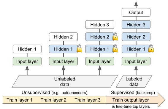
Pre-training on easily labeled data - reuse lower layers for "real" task

Often required due to cost/availability of large labeled datasets
Common tactic: label all training data as "good", generate & corrupt additional instances, label new ones as "bad.

Faster Optimizers

Training speedup strategies thus far: 1) smart weight initializations, 2) smart activation functions, 3) batch normalization, 4) reuse of pretraining.
Better optimizer choices:
- Momentum optimization
- Nesterov Accelerated Gradients
- AdaGrad
- RMSProp
- Adam (should almost always use this one)
Worth noting: below techniques rely on 1st-order partial derivatives (Jacobians); more techniques in literature use 2nd-order derivs (Hessians). Not viable for most deep learning due to memory & computational requirements.

Momentum optimization

local gradient added to a momentum vector (m) multiplied by learning rate (n)
ie, gradient used as an accelerant - not as a speed.
beta hyperparameter serves as friction mechanism. 0 = high friction, 1 = no friction.
Momentum optimization escapes plateaus much faster than GD.

# in TF

optimizer = tf.train.MomentumOptimizer(
    learning_rate=learning_rate,
    momentum=0.9)

Nesterov Accelerated Gradient

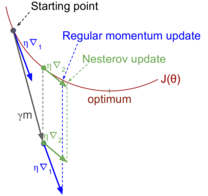
idea: measure cost function gradient slightly ahead in direction of momentum.

# in TF

optimizer = tf.train.MomentumOptimizer(
    learning_rate=learning_rate,
    momentum=0.9, 
    use_nesterov=True)

AdaGrad

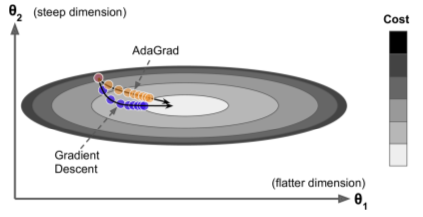
Scales gradient vector along steepest dimensions, ie it decays the learning rate faster for steep dimensions. (ie adaptive learning rate)
Works on simple quadratic problems but often stops too early.

RMSProp

Fixes AdaGrad problem by accumulating most recent gradients (instead of all).
Better than AdaGrad on all but very simple problems. Also better than MO and Nesterov.

# in TF

optimizer = tf.train.RMSPropOptimizer(
    learning_rate=learning_rate,
    momentum=0.9, 
    decay=0.9, 
    epsilon=1e-10)

Adam Optimization (paper:)

Keeps track of decaying past gradients (like Momentum Optimization)
Keeps track of decaying past squared gradients (like RMSProp)
Default params in TF:
Momentum decay param (beta1) usually set to 0.9
Scaling decay param (beta2) usually set to 0.999
Smoothing term (epsilon) usually set to 10e-8

# in TF

optimizer = tf.train.AdamOptimizer(
    learning_rate=learning_rate)

Learning Rate Scheduling

# in TF

initial_learning_rate = 0.1
decay_steps = 10000
decay_rate = 1/10

global_step = tf.Variable(
    0, trainable=False)

learning_rate = tf.train.exponential_decay(
    initial_learning_rate, 
    global_step,
    decay_steps, 
    decay_rate)

optimizer = tf.train.MomentumOptimizer(
    learning_rate, 
    momentum=0.9)

training_op = optimizer.minimize(
    loss, 
    global_step=global_step)

Regularization Techniques

Early Stopping

Simply interrupt training when validation performance starts dropping.

L1 & L2 Regularlization

Dropout

Popular technique - typically adds 1-2% accuracy boost
At every training step, every neuron has probability (p) of being temporarily ignored
Typical p = 50%
In TF: apply dropout() to input layer & output of every hidden layer.

# in TF

from tensorflow.contrib.layers import dropout

[...]

is_training = tf.placeholder(
    tf.bool, 
    shape=(), 
    name='is_training')

keep_prob = 0.5

X_drop = dropout(
    X, 
    keep_prob, 
    is_training=is_training)

hidden1      = fully_connected(
    X_drop, n_hidden1, scope="hidden1")

hidden1_drop = dropout(
    hidden1, keep_prob, is_training=is_training)

hidden2      = fully_connected(
    hidden1_drop, n_hidden2, scope="hidden2")

hidden2_drop = dropout(
    hidden2, keep_prob, is_training=is_training)

logits       = fully_connected(
    hidden2_drop, n_outputs, 
    activation_fn=None,
    scope="outputs")

Max-Norm Regularization

Each neuron's incoming weights are constrained such that ||w||2 <= r
r = max-norm hyperparameter
||.|| = l2 norm
Reducing r increases regularization
Not implemented in TF, but doable.

Data Augmentation

Generating new training instances from existing ones with learnable differences
ex: pics with shifts/rotates/resizes/flips/contrasts
TF has image manipulation ops built-in

Practical Guidelines

Suggested default DNN configurations:
- Initialization: He
- Activation: ELU
- Normalization: Batch
- Regularization: Dropout
- Optimizer: Adam
- Learning Rate schedule: none

ch11 DNN training.md

Vanishing & Exploding Gradients

Xavier & He Initialization

Non-Saturating Activation Functions

Batch Normalization

Batch Normalization with TF

Gradient Clipping

Pretrained Layers & Reuse

Reusing Models from Other Frameworks

Freezing Lower Layers

Caching Lower Layers

Tweaking/Dropping/Replacing Upper Layers

Model Zoos

Unsupervised pre-training

Pre-training on easily labeled data - reuse lower layers for "real" task

Faster Optimizers

Momentum optimization

Nesterov Accelerated Gradient

AdaGrad

RMSProp

Adam Optimization (paper:)

Learning Rate Scheduling

Regularization Techniques

Early Stopping

L1 & L2 Regularlization

Dropout

Max-Norm Regularization

Data Augmentation

Practical Guidelines

results matching ""

No results matching ""