技术分析入门 —— 双均线策略
来源:https://uqer.io/community/share/554051bbf9f06c1c3d687fac
本篇中,我们将通过技术分析流派中经典的“双均线策略”,向大家展现如何在量化实验室中使用Python测试自己的想法,并最终将它转化为策略!
1. 准备工作
一大波Python库需要在使用之前被导入:
matplotlib用于绘制图表numpy时间序列的计算pandas处理结构化的表格数据DataAPI通联数据提供的数据APIseaborn用于美化matplotlib图表
from matplotlib import pylab
import numpy as np
import pandas as pd
import DataAPI
import seaborn as sns
sns.set_style('white')
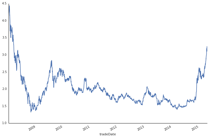
我们的关注点是关于一只ETF基金的投资:华夏上证50ETF,代码:510050.XSHG。我们考虑的回测周期:
- 起始:2008年1月1日
- 结束:2015年4月23日
这里我们使用数据API函数MktFunddGet获取基金交易价格的日线数据,最后获得security是pandas下的DataFrame对象:
secID = '510050.XSHG'
start = '20080101'
end = '20150423'

security = DataAPI.MktFunddGet(secID, beginDate=start, endDate=end, field=['tradeDate', 'closePrice'])
security['tradeDate'] = pd.to_datetime(security['tradeDate'])
security = security.set_index('tradeDate')
security.info()

<class 'pandas.core.frame.DataFrame'>
DatetimeIndex: 1775 entries, 2008-01-02 00:00:00 to 2015-04-23 00:00:00
Data columns (total 1 columns):
closePrice    1775 non-null float64
dtypes: float64(1)
最近5天的收盘价如下:
security.tail()
| closePrice | |
|---|---|
| tradeDate | |
| 2015-04-17 | 3.185 |
| 2015-04-20 | 3.103 |
| 2015-04-21 | 3.141 |
| 2015-04-22 | 3.241 |
| 2015-04-23 | 3.212 |
适当的图表可以帮助研究人员直观的了解标的的历史走势,这里我们直接借助DataFrame的plot成员:
security['closePrice'].plot(grid=False, figsize=(12,8))
sns.despine()
2. 策略描述
这里我们以经典的“双均线”策略为例,讲述如何使用量化实验室进行分析研究。
这里我们使用的均线定义为:
- 短期均线:
window_short = 20,相当于月均线 - 长期均线:
window_long = 120,相当于半年线 - 偏离度阈值:
SD = 5%,区间宽度,这个会在后面有详细解释
计算均值我们借助了numpy的内置移动平均函数:rolling_mean
window_short = 20
window_long = 120
SD = 0.05

security['short_window'] = np.round(pd.rolling_mean(security['closePrice'], window=window_short), 2)
security['long_window'] = np.round(pd.rolling_mean(security['closePrice'], window=window_long), 2)
security[['closePrice', 'short_window', 'long_window']].tail()
| closePrice | short_window | long_window | |
|---|---|---|---|
| tradeDate | |||
| 2015-04-17 | 3.185 | 2.82 | 2.30 |
| 2015-04-20 | 3.103 | 2.85 | 2.31 |
| 2015-04-21 | 3.141 | 2.87 | 2.33 |
| 2015-04-22 | 3.241 | 2.90 | 2.34 |
| 2015-04-23 | 3.212 | 2.93 | 2.35 |
仍然地,我们可以把包含收盘价的三条线画到一张图上,看看有没有什么启发?
security[['closePrice', 'short_window', 'long_window']].plot(grid=False, figsize=(12,8))
sns.despine()

2.1 定义信号
买入信号: 短期均线高于长期日均线,并且超过
SD个点位;卖出信号: 不满足买入信号的所有情况;
我们首先计算短期均线与长期均线的差s-l,这样的向量级运算,在pandas中可以像普通标量一样计算:
security['s-l'] = security['short_window'] - security['long_window']
security['s-l'].tail()

tradeDate
2015-04-17    0.52
2015-04-20    0.54
2015-04-21    0.54
2015-04-22    0.56
2015-04-23    0.58
Name: s-l, dtype: float64
根据s-l的值,我们可以定义信号:
s−l>SD×long_window,支持买入,定义Regime为True- 其他情形下,卖出信号,定义
Regime为False
security['Regime'] = np.where(security['s-l'] > security['long_window'] * SD, 1, 0)
security['Regime'].value_counts()

0    1394
1     381
dtype: int64
上面的统计给出了总共有多少次买入信号,多少次卖出信号。
下图给出了信号的时间分布:
security['Regime'].plot(grid=False, lw=1.5, figsize=(12,8))
pylab.ylim((-0.1,1.1))
sns.despine()

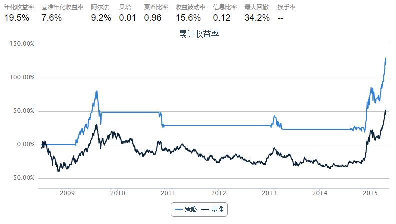
我们可以在有了信号之后执行买入卖出操作,然后根据操作计算每日的收益。这里注意,我们计算策略收益的时候,使用的是当天的信号乘以次日的收益率。这是因为我们的决定是当天做出的,但是能享受到的收益只可能是第二天的(如果用当天信号乘以当日的收益率,那么这里面就有使用未来数据的问题)。
security['Market'] = np.log(security['closePrice'] / security['closePrice'].shift(1))
security['Strategy'] = security['Regime'].shift(1) * security['Market']
security[['Market', 'Strategy', 'Regime']].tail()
| Market | Strategy | Regime | |
|---|---|---|---|
| tradeDate | |||
| 2015-04-17 | 0.012638 | 0.012638 | 1 |
| 2015-04-20 | -0.026083 | -0.026083 | 1 |
| 2015-04-21 | 0.012172 | 0.012172 | 1 |
| 2015-04-22 | 0.031341 | 0.031341 | 1 |
| 2015-04-23 | -0.008988 | -0.008988 | 1 |
最后我们把每天的收益率求和就得到了最后的累计收益率(这里因为我们使用的是指数收益率,所以将每日收益累加是合理的),这个累加的过程也可以通过DataFrame的内置函数cumsum轻松完成:
security[['Market', 'Strategy']].cumsum().apply(np.exp).plot(grid=False, figsize=(12,8))
sns.despine()

3 使用quartz实现策略
上面的部分介绍了从数据出发,在量化实验室内研究策略的流程。实际上我们可以直接用量化实验室内置的quartz框架。quartz框架为用户隐藏了数据获取、数据清晰以及回测逻辑。用户可以更加专注于策略逻辑的描述:
start = datetime(2008, 1, 1)                # 回测起始时间
end  = datetime(2015, 4, 23)                # 回测结束时间
benchmark = 'SH50'                            # 策略参考标准
universe = ['510050.XSHG']    # 股票池
capital_base = 100000     # 起始资金
commission = Commission(0.0,0.0)

window_short = 20
window_long = 120
longest_history = window_long
SD = 0.05

def initialize(account):                    # 初始化虚拟账户状态
    account.fund = universe[0]
    account.SD = SD
    account.window_short = window_short
    account.window_long = window_long

def handle_data(account):             # 每个交易日的买入卖出指令
    hist = account.get_history(longest_history)
    fund = account.fund
    short_mean = np.mean(hist[fund]['closePrice'][-account.window_short:]) # 计算短均线值
    long_mean = np.mean(hist[fund]['closePrice'][-account.window_long:])   #计算长均线值

    # 计算买入卖出信号
    flag = True if (short_mean - long_mean) > account.SD * long_mean else False
    if flag:
        if account.position.secpos.get(fund, 0) == 0:
            # 空仓时全仓买入,买入股数为100的整数倍
            approximationAmount = int(account.cash / hist[fund]['closePrice'][-1]/100.0) * 100
            order(fund, approximationAmount)
    else:
        # 卖出时,全仓清空
        if account.position.secpos.get(fund, 0) >= 0:
            order_to(fund, 0)