实现分解方法
对于这个秘籍,我们将实现一个用于线性回归的矩阵分解方法。具体来说,我们将使用 Cholesky 分解,TensorFlow 中存在相关函数。
做好准备
在大多数情况下,实现前一个秘籍中的逆方法在数值上效率低,尤其是当矩阵变得非常大时。另一种方法是分解A矩阵并对分解执行矩阵运算。一种方法是在 TensorFlow 中使用内置的 Cholesky 分解方法。
人们对将矩阵分解为更多矩阵如此感兴趣的一个原因是,所得到的矩阵将具有允许我们有效使用某些方法的保证属性。 Cholesky 分解将矩阵分解为下三角矩阵和上三角矩阵,比如L和L',使得这些矩阵是彼此的转置。有关此分解属性的更多信息,有许多可用资源来描述它以及如何到达它。在这里,我们将通过将其写为LL'x = b来解决系统Ax = b。我们首先解决Ly = b的y,然后求解L'x = y得到我们的系数矩阵x。
操作步骤
我们按如下方式处理秘籍:
- 我们将以与上一个秘籍完全相同的方式设置系统。我们将导入库,初始化图并创建数据。然后,我们将以之前的方式获得我们的
A矩阵和b矩阵:
import matplotlib.pyplot as plt
import numpy as np
import tensorflow as tf
from tensorflow.python.framework import ops
ops.reset_default_graph()
sess = tf.Session()
x_vals = np.linspace(0, 10, 100)
y_vals = x_vals + np.random.normal(0, 1, 100)
x_vals_column = np.transpose(np.matrix(x_vals))
ones_column = np.transpose(np.matrix(np.repeat(1, 100)))
A = np.column_stack((x_vals_column, ones_column))
b = np.transpose(np.matrix(y_vals))
A_tensor = tf.constant(A)
b_tensor = tf.constant(b)
- 接下来,我们找到方阵的 Cholesky 分解,
A^T A:
tA_A = tf.matmul(tf.transpose(A_tensor), A_tensor)
L = tf.cholesky(tA_A)
tA_b = tf.matmul(tf.transpose(A_tensor), b)
sol1 = tf.matrix_solve(L, tA_b)
sol2 = tf.matrix_solve(tf.transpose(L), sol1)
请注意,TensorFlow 函数
cholesky()仅返回分解的下对角线部分。这很好,因为上对角矩阵只是下对角矩阵的转置。
- 现在我们有了解决方案,我们提取系数:
solution_eval = sess.run(sol2)
slope = solution_eval[0][0]
y_intercept = solution_eval[1][0]
print('slope: ' + str(slope))
print('y_intercept: ' + str(y_intercept))
slope: 0.956117676145
y_intercept: 0.136575513864
best_fit = []
for i in x_vals:
    best_fit.append(slope*i+y_intercept)
plt.plot(x_vals, y_vals, 'o', label='Data')
plt.plot(x_vals, best_fit, 'r-', label='Best fit line', linewidth=3)
plt.legend(loc='upper left')
plt.show()
绘图如下:
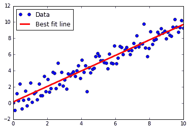
图 2:通过 Cholesky 分解获得的数据点和最佳拟合线
工作原理
如您所见,我们得出了与之前秘籍非常相似的答案。请记住,这种分解矩阵然后对碎片执行操作的方式有时会更加高效和数值稳定,尤其是在考虑大型数据矩阵时。