Powered by GitBook

实现非线性 SVM

对于此秘籍，我们将应用非线性内核来拆分数据集。

做好准备

在本节中，我们将在实际数据上实现前面的高斯核 SVM。我们将加载虹膜数据集并为 I. setosa 创建分类器（与非 setosa 相比）。我们将看到各种伽马值对分类的影响。

操作步骤

我们按如下方式处理秘籍：

我们首先加载必要的库，其中包括scikit-learn数据集，以便我们可以加载虹膜数据。然后，我们将开始图会话。使用以下代码：

import matplotlib.pyplot as plt 
import numpy as np 
import tensorflow as tf 
from sklearn import datasets 
sess = tf.Session()

接下来，我们将加载虹膜数据，提取萼片长度和花瓣宽度，并分离每个类的x和y值（以便以后绘图），如下所示：

iris = datasets.load_iris() 
x_vals = np.array([[x[0], x[3]] for x in iris.data]) 
y_vals = np.array([1 if y==0 else -1 for y in iris.target]) 
class1_x = [x[0] for i,x in enumerate(x_vals) if y_vals[i]==1] 
class1_y = [x[1] for i,x in enumerate(x_vals) if y_vals[i]==1] 
class2_x = [x[0] for i,x in enumerate(x_vals) if y_vals[i]==-1] 
class2_y = [x[1] for i,x in enumerate(x_vals) if y_vals[i]==-1]

现在，我们声明我们的批量大小（首选大批量），占位符和模型变量b，如下所示：

batch_size = 100 

x_data = tf.placeholder(shape=[None, 2], dtype=tf.float32) 
y_target = tf.placeholder(shape=[None, 1], dtype=tf.float32) 
prediction_grid = tf.placeholder(shape=[None, 2], dtype=tf.float32) 

b = tf.Variable(tf.random_normal(shape=[1,batch_size]))

接下来，我们声明我们的高斯内核。这个内核依赖于伽马值，我们将在本文后面的各个伽玛值对分类的影响进行说明。使用以下代码：

gamma = tf.constant(-10.0) 
dist = tf.reduce_sum(tf.square(x_data), 1) 
dist = tf.reshape(dist, [-1,1]) 
sq_dists = tf.add(tf.subtract(dist, tf.multiply(2., tf.matmul(x_data, tf.transpose(x_data)))), tf.transpose(dist)) 
my_kernel = tf.exp(tf.multiply(gamma, tf.abs(sq_dists))) 
# We now compute the loss for the dual optimization problem, as follows: 
model_output = tf.matmul(b, my_kernel) 
first_term = tf.reduce_sum(b) 
b_vec_cross = tf.matmul(tf.transpose(b), b) 
y_target_cross = tf.matmul(y_target, tf.transpose(y_target)) 
second_term = tf.reduce_sum(tf.multiply(my_kernel, tf.multiply(b_vec_cross, y_target_cross))) 
loss = tf.negative(tf.subtract(first_term, second_term))

为了使用 SVM 执行预测，我们必须创建预测内核函数。之后，我们还会声明一个准确率计算，它只是使用以下代码正确分类的点的百分比：

rA = tf.reshape(tf.reduce_sum(tf.square(x_data), 1),[-1,1]) 
rB = tf.reshape(tf.reduce_sum(tf.square(prediction_grid), 1),[-1,1]) 
pred_sq_dist = tf.add(tf.subtract(rA, tf.mul(2., tf.matmul(x_data, tf.transpose(prediction_grid)))), tf.transpose(rB)) 
pred_kernel = tf.exp(tf.multiply(gamma, tf.abs(pred_sq_dist))) 

prediction_output = tf.matmul(tf.multiply(tf.transpose(y_target),b), pred_kernel) 
prediction = tf.sign(prediction_output-tf.reduce_mean(prediction_output)) 
accuracy = tf.reduce_mean(tf.cast(tf.equal(tf.squeeze(prediction), tf.squeeze(y_target)), tf.float32))

接下来，我们声明我们的优化函数并初始化变量，如下所示：

my_opt = tf.train.GradientDescentOptimizer(0.01) 
train_step = my_opt.minimize(loss) 
init = tf.initialize_all_variables() 
sess.run(init)

现在，我们可以开始训练循环了。我们运行循环 300 次迭代并存储损失值和批次精度。为此，我们使用以下实现：

loss_vec = [] 
batch_accuracy = [] 
for i in range(300): 
    rand_index = np.random.choice(len(x_vals), size=batch_size) 
    rand_x = x_vals[rand_index] 
    rand_y = np.transpose([y_vals[rand_index]]) 
    sess.run(train_step, feed_dict={x_data: rand_x, y_target: rand_y}) 

    temp_loss = sess.run(loss, feed_dict={x_data: rand_x, y_target: rand_y}) 
    loss_vec.append(temp_loss) 

    acc_temp = sess.run(accuracy, feed_dict={x_data: rand_x, 
                                             y_target: rand_y, 
                                             prediction_grid:rand_x}) 
    batch_accuracy.append(acc_temp)

为了绘制决策边界，我们将创建x，y点的网格并评估我们在所有这些点上创建的预测函数，如下所示：

x_min, x_max = x_vals[:, 0].min() - 1, x_vals[:, 0].max() + 1 
y_min, y_max = x_vals[:, 1].min() - 1, x_vals[:, 1].max() + 1 
xx, yy = np.meshgrid(np.arange(x_min, x_max, 0.02), 
                     np.arange(y_min, y_max, 0.02)) 
grid_points = np.c_[xx.ravel(), yy.ravel()] 
[grid_predictions] = sess.run(prediction, feed_dict={x_data: x_vals, 
                                                   y_target: np.transpose([y_vals]), 
                                                   prediction_grid: grid_points}) 
grid_predictions = grid_predictions.reshape(xx.shape)

为简洁起见，我们只展示如何用决策边界绘制点。有关 gamma 的图和效果，请参阅本秘籍的下一部分。使用以下代码：

plt.contourf(xx, yy, grid_predictions, cmap=plt.cm.Paired, alpha=0.8) 
plt.plot(class1_x, class1_y, 'ro', label='I. setosa') 
plt.plot(class2_x, class2_y, 'kx', label='Non-setosa') 
plt.title('Gaussian SVM Results on Iris Data') 
plt.xlabel('Petal Length') 
plt.ylabel('Sepal Width') 
plt.legend(loc='lower right') 
plt.ylim([-0.5, 3.0]) 
plt.xlim([3.5, 8.5]) 
plt.show()

工作原理

以下是对四种不同伽玛值（1,10,25 和 100）的 I. setosa 结果的分类。注意伽玛值越高，每个单独点对分类边界的影响越大：

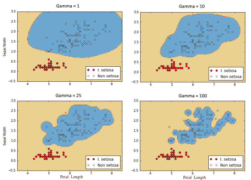
图 9：使用具有四个不同伽马值的高斯核 SVM 的 I. setosa 的分类结果

results matching ""

No results matching ""