实现多类 SVM
我们还可以使用 SVM 对多个类进行分类,而不仅仅是两个类。在本文中,我们将使用多类 SVM 对虹膜数据集中的三种类型的花进行分类。
做好准备
通过设计,SVM 算法是二元分类器。但是,有一些策略可以让他们在多个类上工作。两种主要策略称为“一对一”,“一对一”。
一对一是一种策略,其中为每个可能的类对创建二分类器。然后,对具有最多投票的类的点进行预测。这可能在计算上很难,因为我们必须为k类创建k!/(k - 2)!2!个分类器。
实现多类分类器的另一种方法是执行一对一策略,我们为k类的每个类创建一个分类器。点的预测类将是创建最大 SVM 边距的类。这是我们将在本节中实现的策略。
在这里,我们将加载虹膜数据集并使用高斯内核执行多类非线性 SVM。虹膜数据集是理想的,因为有三个类(setosa,virginica 和 versicolor)。我们将为每个类创建三个高斯核 SVM,并预测存在最高边界的点。
操作步骤
我们按如下方式处理秘籍:
- 首先,我们加载我们需要的库并启动图,如下所示:
import matplotlib.pyplot as plt
import numpy as np
import tensorflow as tf
from sklearn import datasets
sess = tf.Session()
- 接下来,我们将加载虹膜数据集并拆分每个类的目标。我们将仅使用萼片长度和花瓣宽度来说明,因为我们希望能够绘制输出。我们还将每个类的
x和y值分开,以便最后进行绘图。使用以下代码:
iris = datasets.load_iris()
x_vals = np.array([[x[0], x[3]] for x in iris.data])
y_vals1 = np.array([1 if y==0 else -1 for y in iris.target])
y_vals2 = np.array([1 if y==1 else -1 for y in iris.target])
y_vals3 = np.array([1 if y==2 else -1 for y in iris.target])
y_vals = np.array([y_vals1, y_vals2, y_vals3])
class1_x = [x[0] for i,x in enumerate(x_vals) if iris.target[i]==0]
class1_y = [x[1] for i,x in enumerate(x_vals) if iris.target[i]==0]
class2_x = [x[0] for i,x in enumerate(x_vals) if iris.target[i]==1]
class2_y = [x[1] for i,x in enumerate(x_vals) if iris.target[i]==1]
class3_x = [x[0] for i,x in enumerate(x_vals) if iris.target[i]==2]
class3_y = [x[1] for i,x in enumerate(x_vals) if iris.target[i]==2]
- 与实现非线性 SVM 秘籍相比,我们在此示例中所做的最大改变是,许多维度将发生变化(我们现在有三个分类器而不是一个)。我们还将利用矩阵广播和重塑技术一次计算所有三个 SVM。由于我们一次性完成这一操作,我们的
y_target占位符现在具有[3, None]的尺寸,我们的模型变量b将被初始化为[3, batch_size]。使用以下代码:
batch_size = 50

x_data = tf.placeholder(shape=[None, 2], dtype=tf.float32)
y_target = tf.placeholder(shape=[3, None], dtype=tf.float32)
prediction_grid = tf.placeholder(shape=[None, 2], dtype=tf.float32)

b = tf.Variable(tf.random_normal(shape=[3,batch_size]))
- 接下来,我们计算高斯核。由于这仅取决于输入的 x 数据,因此该代码不会改变先前的秘籍。使用以下代码:
gamma = tf.constant(-10.0)
dist = tf.reduce_sum(tf.square(x_data), 1)
dist = tf.reshape(dist, [-1,1])
sq_dists = tf.add(tf.subtract(dist, tf.multiply(2., tf.matmul(x_data, tf.transpose(x_data)))), tf.transpose(dist))
my_kernel = tf.exp(tf.multiply(gamma, tf.abs(sq_dists)))
- 一个重大变化是我们将进行批量矩阵乘法。我们将最终得到三维矩阵,我们将希望在第三个索引上广播矩阵乘法。我们没有为此设置数据和目标矩阵。为了使
x^T · x等操作跨越额外维度,我们创建一个函数来扩展这样的矩阵,将矩阵重新整形为转置,然后在额外维度上调用 TensorFlow 的batch_matmul。使用以下代码:
def reshape_matmul(mat):
    v1 = tf.expand_dims(mat, 1)
    v2 = tf.reshape(v1, [3, batch_size, 1])
    return tf.batch_matmul(v2, v1)
- 创建此函数后,我们现在可以计算双重损失函数,如下所示:
model_output = tf.matmul(b, my_kernel)
first_term = tf.reduce_sum(b)
b_vec_cross = tf.matmul(tf.transpose(b), b)
y_target_cross = reshape_matmul(y_target)

second_term = tf.reduce_sum(tf.multiply(my_kernel, tf.multiply(b_vec_cross, y_target_cross)),[1,2])
loss = tf.reduce_sum(tf.negative(tf.subtract(first_term, second_term)))
- 现在,我们可以创建预测内核。请注意,我们必须小心
reduce_sum函数并且不要在所有三个 SVM 预测中减少,因此我们必须告诉 TensorFlow 不要用第二个索引参数对所有内容求和。使用以下代码:
rA = tf.reshape(tf.reduce_sum(tf.square(x_data), 1),[-1,1])
rB = tf.reshape(tf.reduce_sum(tf.square(prediction_grid), 1),[-1,1])
pred_sq_dist = tf.add(tf.subtract(rA, tf.multiply(2., tf.matmul(x_data, tf.transpose(prediction_grid)))), tf.transpose(rB))
pred_kernel = tf.exp(tf.multiply(gamma, tf.abs(pred_sq_dist)))
- 当我们完成预测内核时,我们可以创建预测。这里的一个重大变化是预测不是输出的
sign()。由于我们正在实现一对一策略,因此预测是具有最大输出的分类器。为此,我们使用 TensorFlow 的内置argmax()函数,如下所示:
prediction_output = tf.matmul(tf.mul(y_target,b), pred_kernel)
prediction = tf.arg_max(prediction_output-tf.expand_dims(tf.reduce_mean(prediction_output,1), 1), 0)
accuracy = tf.reduce_mean(tf.cast(tf.equal(prediction, tf.argmax(y_target,0)), tf.float32))
- 现在我们已经拥有了内核,损失和预测函数,我们只需要声明我们的优化函数并初始化我们的变量,如下所示:
my_opt = tf.train.GradientDescentOptimizer(0.01)
train_step = my_opt.minimize(loss)
init = tf.global_variables_initializer()
sess.run(init)
- 该算法收敛速度相对较快,因此我们不必运行训练循环超过 100 次迭代。我们使用以下代码执行此操作:
loss_vec = []
batch_accuracy = []
for i in range(100):
    rand_index = np.random.choice(len(x_vals), size=batch_size)
    rand_x = x_vals[rand_index]
    rand_y = y_vals[:,rand_index]
    sess.run(train_step, feed_dict={x_data: rand_x, y_target: rand_y})

    temp_loss = sess.run(loss, feed_dict={x_data: rand_x, y_target: rand_y})
    loss_vec.append(temp_loss)

    acc_temp = sess.run(accuracy, feed_dict={x_data: rand_x, y_target: rand_y, prediction_grid:rand_x})
    batch_accuracy.append(acc_temp)

    if (i+1)%25==0:
        print('Step #' + str(i+1))
        print('Loss = ' + str(temp_loss))

Step #25
Loss = -2.8951
Step #50
Loss = -27.9612
Step #75
Loss = -26.896
Step #100
Loss = -30.2325
- 我们现在可以创建点的预测网格并对所有点运行预测函数,如下所示:
x_min, x_max = x_vals[:, 0].min() - 1, x_vals[:, 0].max() + 1
y_min, y_max = x_vals[:, 1].min() - 1, x_vals[:, 1].max() + 1
xx, yy = np.meshgrid(np.arange(x_min, x_max, 0.02),
                     np.arange(y_min, y_max, 0.02))
grid_points = np.c_[xx.ravel(), yy.ravel()]
grid_predictions = sess.run(prediction, feed_dict={x_data: rand_x,
                                                   y_target: rand_y,
                                                   prediction_grid: grid_points})
grid_predictions = grid_predictions.reshape(xx.shape)
- 以下是绘制结果,批量准确率和损失函数的代码。为简洁起见,我们只显示最终结果:
plt.contourf(xx, yy, grid_predictions, cmap=plt.cm.Paired, alpha=0.8)
plt.plot(class1_x, class1_y, 'ro', label='I. setosa')
plt.plot(class2_x, class2_y, 'kx', label='I. versicolor')
plt.plot(class3_x, class3_y, 'gv', label='I. virginica')
plt.title('Gaussian SVM Results on Iris Data')
plt.xlabel('Petal Length')
plt.ylabel('Sepal Width')
plt.legend(loc='lower right')
plt.ylim([-0.5, 3.0])
plt.xlim([3.5, 8.5])
plt.show()

plt.plot(batch_accuracy, 'k-', label='Accuracy')
plt.title('Batch Accuracy')
plt.xlabel('Generation')
plt.ylabel('Accuracy')
plt.legend(loc='lower right')
plt.show()

plt.plot(loss_vec, 'k-')
plt.title('Loss per Generation')
plt.xlabel('Generation')
plt.ylabel('Loss')
plt.show()
然后我们得到以下绘图:
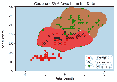
图 10:在伽马= 10 的虹膜数据集上的多类(三类)非线性高斯 SVM 结果
我们观察前面的屏幕截图,其中显示了所有三个虹膜类,以及为每个类分类的点网格。
工作原理
本文中需要注意的重点是我们如何改变算法以同时优化三个 SVM 模型。我们的模型参数b有一个额外的维度可以考虑所有三个模型。在这里,我们可以看到,由于 TensorFlow 处理额外维度的内置函数,算法扩展到多个类似算法相对容易。
下一章将介绍最近邻方法,这是一种用于预测目的的非常强大的算法。