学习 TensorFlow 线性回归方法

虽然使用矩阵和分解方法非常强大，但 TensorFlow 还有另一种解决斜率和截距的方法。 TensorFlow 可以迭代地执行此操作，逐步学习最小化损失的线性回归参数。

做好准备

在这个秘籍中，我们将遍历批量数据点并让 TensorFlow 更新斜率和y截距。我们将使用内置于 scikit-learn 库中的 iris 数据集，而不是生成的数据。具体来说，我们将通过数据点找到最佳线，其中x值是花瓣宽度，y值是萼片长度。我们选择了这两个，因为它们之间似乎存在线性关系，我们将在最后的绘图中看到。我们还将在下一节中详细讨论不同损失函数的影响，但对于这个秘籍，我们将使用 L2 损失函数。

操作步骤

我们按如下方式处理秘籍：

1. 我们首先加载必要的库，创建图并加载数据：

import matplotlib.pyplot as plt 
import numpy as np 
import tensorflow as tf 
from sklearn import datasets 
from tensorflow.python.framework import ops 
ops.reset_default_graph() 
sess = tf.Session() 
iris = datasets.load_iris() 
x_vals = np.array([x[3] for x in iris.data]) 
y_vals = np.array([y[0] for y in iris.data])

1. 然后我们声明我们的学习率，批量大小，占位符和模型变量：

learning_rate = 0.05 
batch_size = 25 
x_data = tf.placeholder(shape=[None, 1], dtype=tf.float32) 
y_target = tf.placeholder(shape=[None, 1], dtype=tf.float32) 
A = tf.Variable(tf.random_normal(shape=[1,1])) 
b = tf.Variable(tf.random_normal(shape=[1,1]))

1. 接下来，我们编写线性模型的公式y = Ax + b：

model_output = tf.add(tf.matmul(x_data, A), b)

1. 然后，我们声明我们的 L2 损失函数（包括批量的平均值），初始化变量，并声明我们的优化器。请注意，我们选择0.05作为我们的学习率：

loss = tf.reduce_mean(tf.square(y_target - model_output)) 
init = tf.global_variables_initializer() 
sess.run(init) 
my_opt = tf.train.GradientDescentOptimizer(learning_rate) 
train_step = my_opt.minimize(loss)

1. 我们现在可以在随机选择的批次上循环并训练模型。我们将运行 100 个循环并每 25 次迭代打印出变量和损失值。请注意，在这里，我们还保存了每次迭代的损失，以便我们以后可以查看它们：

loss_vec = [] 
for i in range(100): 
    rand_index = np.random.choice(len(x_vals), size=batch_size) 
    rand_x = np.transpose([x_vals[rand_index]]) 
    rand_y = np.transpose([y_vals[rand_index]]) 
    sess.run(train_step, feed_dict={x_data: rand_x, y_target: rand_y}) 
    temp_loss = sess.run(loss, feed_dict={x_data: rand_x, y_target: rand_y}) 
    loss_vec.append(temp_loss) 
    if (i+1)%25==0: 
        print('Step #' + str(i+1) + ' A = ' + str(sess.run(A)) + ' b = ' + str(sess.run(b))) 
        print('Loss = ' + str(temp_loss)) 

Step #25 A = [[ 2.17270374]] b = [[ 2.85338426]] 
Loss = 1.08116 
Step #50 A = [[ 1.70683455]] b = [[ 3.59916329]] 
Loss = 0.796941 
Step #75 A = [[ 1.32762754]] b = [[ 4.08189011]] 
Loss = 0.466912 
Step #100 A = [[ 1.15968263]] b = [[ 4.38497639]] 
Loss = 0.281003

1. 接下来，我们将提取我们找到的系数并创建一个最合适的线以放入图中：

[slope] = sess.run(A) 
[y_intercept] = sess.run(b) 
best_fit = [] 
for i in x_vals: 
    best_fit.append(slope*i+y_intercept)

1. 在这里，我们将创建两个图。第一个是覆盖拟合线的数据。第二个是 100 次迭代中的 L2 损失函数。这是生成两个图的代码。

plt.plot(x_vals, y_vals, 'o', label='Data Points') 
plt.plot(x_vals, best_fit, 'r-', label='Best fit line', linewidth=3) 
plt.legend(loc='upper left') 
plt.title('Sepal Length vs Petal Width') 
plt.xlabel('Petal Width') 
plt.ylabel('Sepal Length') 
plt.show() 
plt.plot(loss_vec, 'k-') 
plt.title('L2 Loss per Generation') 
plt.xlabel('Generation') 
plt.ylabel('L2 Loss') 
plt.show()

此代码生成以下拟合数据和损失图。

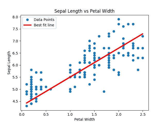
图 3：来自虹膜数据集的数据点（萼片长度与花瓣宽度）重叠在 TensorFlow 中找到的最佳线条拟合。

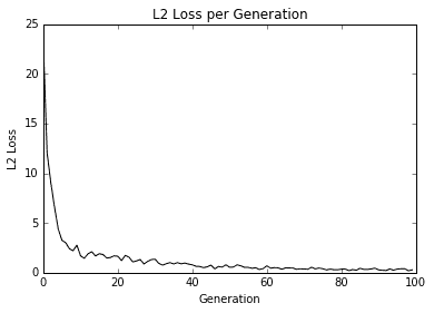
图 4：用我们的算法拟合数据的 L2 损失;注意损失函数中的抖动，可以通过较大的批量大小减小抖动，或者通过较小的批量大小来增加。

Here is a good place to note how to see whether the model is overfitting or underfitting the data. If our data is broken into test and training sets, and the accuracy is greater on the training set and lower on the test set, then we are overfitting the data. If the accuracy is still increasing on both test and training sets, then the model is underfitting and we should continue training.

工作原理

找到的最佳线不保证是最合适的线。最佳拟合线的收敛取决于迭代次数，批量大小，学习率和损失函数。随着时间的推移观察损失函数总是很好的做法，因为它可以帮助您解决问题或超参数变化。