使用最近邻
我们将通过实现最近邻来预测住房价值来开始本章。这是从最近邻居开始的好方法,因为我们将处理数字特征和连续目标。
做好准备
为了说明如何在 TensorFlow 中使用最近邻居进行预测,我们将使用波士顿住房数据集。在这里,我们将预测邻域住房价值中位数作为几个特征的函数。
由于我们考虑训练集训练模型,我们将找到预测点的 k-NN,并将计算目标值的加权平均值。
操作步骤
我们按如下方式处理秘籍:
- 我们将从加载所需的库并开始图会话开始。我们将使用
requests模块从 UCI 机器学习库加载必要的波士顿住房数据:
import matplotlib.pyplot as plt
import numpy as np
import tensorflow as tf
import requests

sess = tf.Session()
- 接下来,我们将使用
requests模块加载数据:
housing_url = 'https://archive.ics.uci.edu/ml/machine-learning-databases/housing/housing.data'
housing_header = ['CRIM', 'ZN', 'INDUS', 'CHAS', 'NOX', 'RM', 'AGE', 'DIS', 'RAD', 'TAX', 'PTRATIO', 'B', 'LSTAT', 'MEDV']
cols_used = ['CRIM', 'INDUS', 'NOX', 'RM', 'AGE', 'DIS', 'TAX', 'PTRATIO', 'B', 'LSTAT']
num_features = len(cols_used)
# Request data
housing_file = requests.get(housing_url)
# Parse Data
housing_data = [[float(x) for x in y.split(' ') if len(x)>=1] for y in housing_file.text.split('n') if len(y)>=1]
- 接下来,我们将数据分为依赖和独立的特征。我们将预测最后一个变量
MEDV,这是房屋组的中值。我们也不会使用ZN,CHAS和RAD特征,因为它们没有信息或二元性质:
y_vals = np.transpose([np.array([y[13] for y in housing_data])])
x_vals = np.array([[x for i,x in enumerate(y) if housing_header[i] in cols_used] for y in housing_data])

x_vals = (x_vals - x_vals.min(0)) / x_vals.ptp(0)
- 现在,我们将
x和y值分成训练和测试集。我们将通过随机选择大约 80%的行来创建训练集,并将剩下的 20%留给测试集:
train_indices = np.random.choice(len(x_vals), round(len(x_vals)*0.8), replace=False)
test_indices = np.array(list(set(range(len(x_vals))) - set(train_indices)))
x_vals_train = x_vals[train_indices]
x_vals_test = x_vals[test_indices]
y_vals_train = y_vals[train_indices]
y_vals_test = y_vals[test_indices]
- 接下来,我们将声明
k值和批量大小:
k = 4
batch_size=len(x_vals_test)
- 我们接下来会申报占位符。请记住,没有模型变量需要训练,因为模型完全由我们的训练集确定:
x_data_train = tf.placeholder(shape=[None, num_features], dtype=tf.float32)
x_data_test = tf.placeholder(shape=[None, num_features], dtype=tf.float32)
y_target_train = tf.placeholder(shape=[None, 1], dtype=tf.float32)
y_target_test = tf.placeholder(shape=[None, 1], dtype=tf.float32)
- 接下来,我们将为一批测试点创建距离函数。在这里,我们将说明 L1 距离的使用:
distance = tf.reduce_sum(tf.abs(tf.subtract(x_data_train, tf.expand_dims(x_data_test,1))), reduction_indices=2)
注意,也可以使用 L2 距离函数。我们将距离公式改为
distance = tf.sqrt(tf.reduce_sum(tf.square(tf.subtract(x_data_train, tf.expand_dims(x_data_test,1))), reduction_indices=1))。
- 现在,我们将创建我们的预测函数。为此,我们将使用
top_k()函数,该函数返回张量中最大值的值和索引。由于我们想要最小距离的指数,我们将找到k- 最大负距离。我们还将声明目标值的预测和均方误差(MSE):
top_k_xvals, top_k_indices = tf.nn.top_k(tf.negative(distance), k=k)
x_sums = tf.expand_dims(tf.reduce_sum(top_k_xvals, 1),1)
x_sums_repeated = tf.matmul(x_sums,tf.ones([1, k], tf.float32))
x_val_weights = tf.expand_dims(tf.divide(top_k_xvals,x_sums_repeated), 1)

top_k_yvals = tf.gather(y_target_train, top_k_indices)
prediction = tf.squeeze(tf.batch_matmul(x_val_weights,top_k_yvals), squeeze_dims=[1])
mse = tf.divide(tf.reduce_sum(tf.square(tf.subtract(prediction, y_target_test))), batch_size)
- 现在,我们将遍历测试数据并存储预测和准确率值:
num_loops = int(np.ceil(len(x_vals_test)/batch_size))

for i in range(num_loops):
    min_index = i*batch_size
    max_index = min((i+1)*batch_size,len(x_vals_train))
    x_batch = x_vals_test[min_index:max_index]
    y_batch = y_vals_test[min_index:max_index]
    predictions = sess.run(prediction, feed_dict={x_data_train: x_vals_train, x_data_test: x_batch, y_target_train: y_vals_train, y_target_test: y_batch})
    batch_mse = sess.run(mse, feed_dict={x_data_train: x_vals_train, x_data_test: x_batch, y_target_train: y_vals_train, y_target_test: y_batch})

    print('Batch #' + str(i+1) + ' MSE: ' + str(np.round(batch_mse,3)))

Batch #1 MSE: 23.153
- 另外,我们可以查看实际目标值与预测值的直方图。看待这一点的一个原因是要注意这样一个事实:使用平均方法,我们无法预测目标的极端:
bins = np.linspace(5, 50, 45)
plt.hist(predictions, bins, alpha=0.5, label='Prediction')
plt.hist(y_batch, bins, alpha=0.5, label='Actual')
plt.title('Histogram of Predicted and Actual Values')
plt.xlabel('Med Home Value in $1,000s')
plt.ylabel('Frequency')
plt.legend(loc='upper right')
plt.show()
然后我们将获得直方图,如下所示:
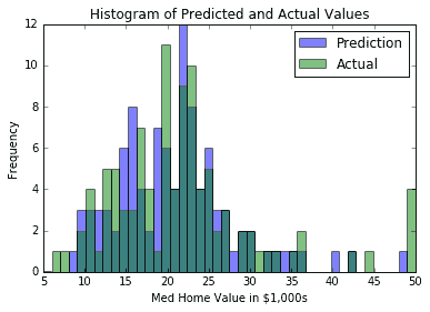
图 1:k-NN 的预测值和实际目标值的直方图(其中k=4)
一个难以确定的是k的最佳价值。对于上图和预测,我们将k=4用于我们的模型。我们之所以选择这个,是因为它给了我们最低的 MSE。这通过交叉验证来验证。如果我们在k的多个值上使用交叉验证,我们将看到k=4给我们一个最小的 MSE。我们在下图中说明了这一点。绘制预测值的方差也是值得的,以表明它会随着我们平均的邻居越多而减少:
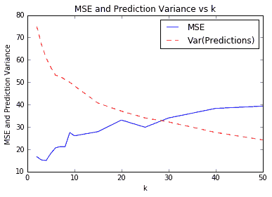
图 2:各种k值的 k-NN 预测的 MSE。我们还绘制了测试集上预测值的方差。请注意,随着k的增加,方差会减小。
工作原理
使用最近邻算法,模型是训练集。因此,我们不必在模型中训练任何变量。唯一的参数k是通过交叉验证确定的,以最大限度地减少我们的 MSE。
更多
对于 k-NN 的加权,我们选择直接按距离加权。还有其他选择我们也可以考虑。另一种常见方法是通过反平方距离加权。